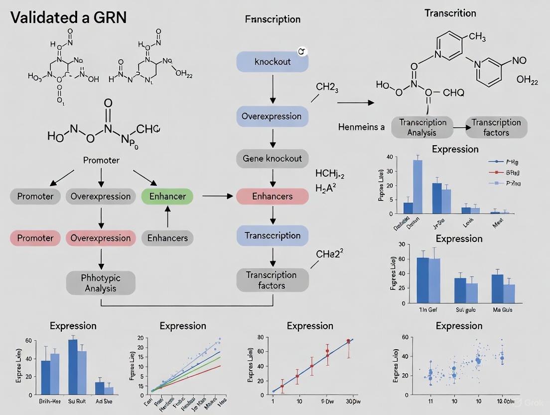
Validating Gene Regulatory Network Models: A Guide to Functional Experiments and Best Practices

Abstract

This article provides a comprehensive guide for researchers and drug development professionals on validating Gene Regulatory Network (GRN) models through functional experiments. It covers the foundational principles of GRN validation, explores a range of methodological approaches from perturbation assays to multi-omic integration, addresses common troubleshooting and optimization challenges, and establishes frameworks for rigorous validation and comparative analysis. By synthesizing current methodologies and emerging trends, this resource aims to equip scientists with the knowledge to robustly test and refine their GRN models, thereby enhancing the reliability of insights for basic research and therapeutic development.

The Bedrock of Belief: Core Principles and Exploratory Techniques for GRN Validation

GRN Validation FAQs: Addressing Key Experimental Challenges

FAQ 1: Our inferred GRN shows poor correlation with experimental co-expression data. How can we validate the model's predictive power?

A high-quality GRN model should recapitulate experimentally observed gene expression relationships. To validate this, you can employ the Fokker-Planck equation methodology to derive a theoretical co-expression matrix from your dynamical GRN model and compare it directly to experimental data [1]. The protocol involves:

• Obtain the stationary solution of the Fokker-Planck equation for your GRN model, which represents the probability distribution of gene expression states.
• Calculate the theoretical co-expression matrix from this stationary solution.
• Perform quantitative comparison against the experimental co-expression matrix using correlation metrics. Studies on the Arabidopsis thaliana flower morphogenesis network have shown good agreement between theoretical and experimental matrices, confirming model accuracy [1].

FAQ 2: How can we prioritize which transcription factors (TFs) to validate first from a large set of computationally predicted regulators?

To efficiently prioritize key regulators from a large set of candidates, use a method that combines robust transcription factor activity (TFA) estimation with model-guided experimental design [2]. The process involves:

• Apply prior knowledge-guided sparsity regularization (e.g., MERLIN+P+TFA method) to your bulk or single-cell data to robustly estimate TFA and infer GRNs, which helps mitigate noise in prior knowledge [2].
• Use the inferred network structure to rank regulators based on their predicted importance in the network.
• Experimentally validate the top-prioritized regulators. This approach has been successfully used to validate 58 key regulators in mouse Embryonic Stem Cells (mECS), identifying both known and novel regulators of the mESC state [2].

FAQ 3: Our single-cell data is sparse and highly heterogeneous. How does this affect GRN inference and validation?

Single-cell RNA sequencing (scRNA-seq) data sparsity and cellular heterogeneity present significant challenges that can obscure true gene-gene relationships. To address this:

• Employ advanced computational frameworks like HyperG-VAE, a hypergraph variational autoencoder, which enhances scRNA-seq representation by reducing sparsity effects and capturing latent correlations among genes and cells [3].
• This method specifically models cellular heterogeneity and identifies gene modules, leading to more accurate GRN predictions from heterogeneous single-cell data as demonstrated in B cell development studies [3].
• Focus validation efforts on regulatory relationships that are consistently predicted across cell states or within identified cell clusters.

FAQ 4: What constitutes a "validated" GRN model versus a predictive one, and how do validation standards differ?

A predictive GRN model identifies potential regulatory relationships, while a validated model confirms these connections with functional biological evidence. Key differences include:

• Computational Prediction: Relies on statistical associations from expression data (e.g., co-expression) and may incorporate prior knowledge. The quality is benchmarked against known networks or simulation [2] [3].
• Biological Validation: Requires experimental confirmation that a transcription factor directly or indirectly regulates a target gene, influencing a biological function or phenotype. It is crucial to generate context-specific gold standards for validation, as computationally inferred networks can capture functional targets with higher precision than estimated in general benchmarks [2].

FAQ 5: Can AI-designed tools improve the experimental validation of GRN predictions?

Yes, AI-designed molecular tools can significantly enhance validation experiments. For instance, large language models trained on biological sequences can now generate highly functional, novel gene editors [4].

• Application: These AI-generated editors (e.g., OpenCRISPR-1) enable precise perturbation of predicted regulatory elements (e.g., TF genes, enhancers) to test their functional impact on target genes within the GRN [4].
• Advantage: They often exhibit comparable or improved activity and specificity relative to naturally derived editors like SpCas9, providing more reliable tools for functional validation in human cells and other systems [4].

GRN Validation Techniques: Methodologies and Data

Table 1: Summary of Computational Methods for GRN Inference and Validation

Method Name	Core Principle	Data Type	Key Validation Metric	Reported Outcome
MERLIN+P+TFA [2]	Robust TFA estimation using prior knowledge-guided sparsity regularization.	Bulk & Single-Cell	Precision of prioritized TF targets vs. experimental validation.	Identified & validated 58 regulators in mESC; captured functional targets with high precision.
Fokker-Planck Equation (FPE) [1]	Models epigenetic landscape & stationary gene expression distribution.	Pre-defined GRN Topology	Correlation between theoretical and experimental co-expression matrices.	Good agreement with experimental co-expression in Arabidopsis thaliana flower morphogenesis.
HyperG-VAE [3]	Hypergraph learning to model cellular heterogeneity and gene modules.	scRNA-seq	Benchmarking against known networks; Gene set enrichment analysis.	Excelled in GRN prediction, single-cell clustering, and lineage tracing in B cell data.

Table 2: Essential Research Reagent Solutions for GRN Validation

Reagent / Tool	Function in GRN Validation	Key Feature / Application
Validated TF Perturbation Tools (e.g., CRISPRi/a, siRNA)	Experimentally modulate the activity of a predicted TF to observe changes in target gene expression.	Essential for establishing causal regulatory relationships.
AI-Designed Gene Editors (e.g., OpenCRISPR-1) [4]	Precision editing of genomic regulatory elements with high specificity and activity.	Useful for validating TF binding sites and enhancer-promoter interactions.
Context-Specific Gold Standard Datasets [2]	A set of previously confirmed TF-target interactions specific to the cell type or condition being studied.	Serves as a critical benchmark for evaluating the accuracy of a newly inferred GRN.

Experimental Protocols for Key Validation Steps

Protocol 1: Validating TF-Target Relationships Using Knockdown and RT-qPCR

This fundamental protocol tests whether reducing a predicted TF's level leads to expression changes in its putative target genes.

• Perturbation: Using siRNA or CRISPR interference (CRISPRi), knock down the expression of the prioritized TF in your cell model.
• Validation of Knockdown: 48-72 hours post-transfection, harvest cells. Isolate RNA and synthesize cDNA. Perform RT-qPCR to confirm successful reduction of the TF's mRNA.
• Target Gene Analysis: Using the same cDNA samples, measure the expression levels of the predicted target genes via RT-qPCR.
• Data Interpretation: A significant decrease (for an activating TF) or increase (for a repressive TF) in the expression of the target genes confirms a functional regulatory relationship. Always include appropriate negative controls (e.g., non-targeting siRNA).

Protocol 2: Model Validation via the Fokker-Planck Equation

This advanced computational protocol validates whether a GRN model can generate biologically realistic gene expression patterns [1].

• Formulate the Dynamical System: Define a continuous-time dynamical system (e.g., a system of ordinary differential equations) that describes the temporal evolution of protein concentrations in your GRN.
• Construct the Fokker-Planck Equation (FPE): Formulate the FPE associated with your dynamical system to describe the time evolution of the probability distribution over all possible expression states.
• Solve for Stationary Distribution: Obtain the stationary solution of the FPE, which represents the long-term probability distribution of the network's states (the "epigenetic landscape"). Numerical methods, such as a gamma mixture model, can be used to approximate this solution [1].
• Calculate Theoretical Co-expression: From the stationary distribution, compute the theoretical covariance or correlation matrix between all genes in the network.
• Compare with Experiment: Quantitatively compare this theoretical co-expression matrix to an experimentally derived co-expression matrix from your biological system. A strong correlation supports the validity of your GRN model.

GRN Validation Workflow and Pathway Diagrams

GRN Validation Workflow

This diagram outlines the core iterative cycle for validating a Gene Regulatory Network (GRN), integrating both computational refinement and essential experimental steps.

FPE Model Validation

This diagram details the specific pathway for validating a GRN model by comparing its theoretical predictions against real experimental data using the Fokker-Planck equation.

Welcome to the GRN Validation Support Center

This resource provides troubleshooting guides and FAQs for researchers validating Gene Regulatory Network models through functional experiments. Here, you will find solutions for common challenges in linking computational predictions to phenotypic outcomes.

Frequently Asked Questions & Troubleshooting

Q1: My inferred GRN shows high computational accuracy (e.g., AUROC), but fails to predict phenotypic outcomes in validation experiments. What could be wrong?

• Potential Cause 1: Disconnect between mRNA and protein-level regulation. The Central Dogma involves both transcription and translation, and regulatory interactions often occur at the protein level. A model based solely on transcriptomic data (e.g., scRNA-seq) may miss key post-transcriptional regulatory mechanisms [5] [6].

  • Solution: Whenever possible, incorporate proteomic data. If high-throughput proteomics is not feasible, use targeted experiments (e.g., Western blot, ELISA) to validate the protein abundance of key predicted regulators and targets.

• Potential Cause 2: Overfitting to expression data without biological constraints. The model may have learned technical or biological noise specific to your dataset rather than generalizable regulatory principles [7].

  • Solution: Integrate prior knowledge into your model. "Prune" your network using high-confidence, experimentally validated interactions from databases. Use precision-recall analysis against known interactions to set a confidence threshold for your predictions, keeping only edges above this threshold [8].

Q2: How can I validate a GRN model when a full "gold standard" network for my biological system is unavailable?

• Solution: Employ a network shuffling and cross-validation protocol.
  • Generate a null distribution by shuffling the links of your inferred GRN while preserving network properties like node in-degree [9].
  • Fit both your original inferred GRN and the shuffled networks to your training data under cross-validation.
  • Calculate a goodness-of-fit measure, such as the weighted Residual Sum of Squares (wRSS), for both the true and shuffled networks.
  • Compare your model's wRSS against the null distribution. A model that fits significantly better than its shuffled counterparts provides confidence in its predictive power, even without a complete gold standard [9].

Q3: The perturbation experiments I designed (e.g., knockdown) do not show the expected effects on my GRN model's predicted targets. How should I troubleshoot this?

• Potential Cause: The effective perturbation design is obfuscated by experimental noise or off-target effects. The intended perturbation matrix may not accurately reflect the actual perturbations captured in the gene expression data due to experimental artifacts [10].
  • Solution: Infer the effective perturbation design directly from the gene expression data. Tools like IDEMAX use a Z-score approach to identify which experiments show significant expression changes for each gene, creating a perturbation matrix that better reflects the data's reality. Using this inferred matrix for GRN inference can improve accuracy [10].

Q4: How do I move from a list of correlated genes to a causal GRN that can be tested functionally?

• Solution: A stepwise inference and validation pipeline.
  • Identify phenotype-associated genes: Use methods like Weighted Gene Co-expression Network Analysis (WGCNA) to find gene modules highly correlated with your phenotypic data [8].
  • Infer regulators: Focus on Transcription Factors (TFs) within these key modules.
  • Predict genome-wide targets: Use a network inference algorithm (e.g., GENIE3, a random-forest based method) to predict the targets for your candidate TFs [8].
  • Prune for high-confidence interactions: Validate and "prune" the initial network by comparing TF→target predictions against independent, high-confidence validation datasets (e.g., from ChIP-seq or other functional assays). Set a precision threshold to keep only the most reliable edges [8].

Essential Metrics for GRN Validation

The table below summarizes key quantitative metrics used to evaluate GRN inference methods.

Table 1: Key Quantitative Metrics for GRN Inference Evaluation

Metric	Formula/Description	Interpretation
AUROC (Area Under the Receiver Operating Characteristic Curve)	Plots True Positive Rate (TPR) against False Positive Rate (FPR) across all prediction confidence thresholds [5].	A perfect score is 1.0. An AUROC of 0.5 indicates performance equivalent to random guessing. Measures the ability to distinguish true edges from non-edges overall [5].
AUPR (Area Under the Precision-Recall Curve)	Plots Precision (Positive Predictive Value) against Recall (True Positive Rate) across all thresholds [8].	Often more informative than AUROC for highly imbalanced datasets (where true edges are rare). A higher AUPR indicates better performance.
True Positive Rate (TPR) / Recall	( TPR = \frac{TP}{TP + FN} )	The proportion of actual true edges that were correctly identified [5].
False Positive Rate (FPR)	( FPR = \frac{FP}{FP + TN} )	The proportion of actual non-edges that were incorrectly predicted as edges [5].
Precision	( Precision = \frac{TP}{TP + FP} )	The proportion of predicted edges that are actually true edges. Critical for assessing the usability of a network for costly experimental validation [8].

Detailed Experimental Protocols

Protocol 1: Validating a GRN's Topology Without a Gold Standard

This protocol uses a Monte Carlo sampling approach to build a null distribution for comparing your inferred GRN's goodness-of-fit [9].

• Infer GRN Topology: Use your chosen method (e.g., GENIE3, LASSO, etc.) to infer a network from your gene expression data. This is your inferred GRN.
• Generate Null GRNs: Create a set of shuffled networks by randomly rewiring the links of your inferred GRN. Preserve the in-degree of each node to maintain the hub structure of the original network [9].
• Fit to Training Data: Under cross-validation, fit both your inferred GRN and the shuffled null GRNs to your original training data. Use a method that balances measurement and process errors during this fitting process [9].
• Calculate Goodness-of-Fit: For each network (inferred and null), calculate a weighted Residual Sum of Squares (wRSS) or a similar error metric that reflects its ability to predict the data.
• Compare Against Null Distribution: Statistically compare the wRSS of your inferred GRN against the distribution of wRSS from the null GRNs. A significantly lower wRSS for your model indicates a topology that is more predictive than random chance [9].

Protocol 2: Pruning a GRN for High-Confidence Experimental Validation

This protocol describes how to refine a large, computationally inferred network to a high-confidence subset of interactions suitable for functional testing [8].

• Initial Network Inference: Start with a list of TFs of interest and perform genome-wide target prediction using an inference tool like GENIE3. This generates a large, unrefined network with many potential edges.
• Gather Validation Datasets: Collect independent, high-confidence experimental data for at least some TFs in your network. This can include in planta RNA-seq after TF perturbation or ChIP-seq data for direct binding targets [8].
• Precision-Recall Analysis: For the TFs with validation data, perform a Precision-Recall analysis. Plot the precision against the recall of your GENIE3 predictions at different score thresholds.
• Set a Precision Cut-off: Analyze the Precision-Recall curve to determine a score threshold that achieves an acceptable level of precision (e.g., 0.31, as used in one study [8]). This threshold represents a trade-off between the number of predictions (recall) and their reliability (precision).
• Prune the Network: Apply this score threshold to the entire inferred network. Remove all predicted TF→target edges with scores below the threshold. The resulting "pruned" network contains a smaller set of high-confidence predictions for downstream experimental validation.

Workflow and Pathway Visualizations

GRN Validation Workflow

GRN Inference & Evaluation Framework

The Scientist's Toolkit: Research Reagent Solutions

Table 2: Essential Reagents and Resources for GRN Validation Experiments

Item	Function in GRN Validation	Example Use Case
Single-cell Multi-ome ATAC + Gene Expression	Simultaneously profiles chromatin accessibility (ATAC-seq) and gene expression (RNA-seq) in the same single cell [11].	Identifies putative enhancer/gene pairs and links TF binding sites to target gene expression at a cellular resolution.
ChIP-seq Grade Antibodies	Antibodies specific to TFs or histone modifications for Chromatin Immunoprecipitation followed by sequencing (ChIP-seq) [11].	Validates the physical binding of a predicted TF regulator to the genomic regions of its target genes.
CRISPR Activation/Interference (CRISPRa/i)	Tools for targeted gene overexpression (activation) or knockdown (interference) without altering the DNA sequence itself.	Functionally tests the predicted causal effect of a TF on its target genes and the resulting phenotypic outcome.
Perturbation Vectors (shRNA, siRNA)	Constructs for targeted gene knockdown (loss-of-function) in perturbation experiments [10].	Tests the necessity of a predicted regulator for the expression of its target genes and for a specific phenotype.
GENIE3	A random forest-based network inference algorithm to predict the targets of transcription factors [8].	Generates an initial, genome-wide set of TF→target predictions from gene expression data.
WGCNA	A bioinformatic algorithm for finding clusters (modules) of highly correlated genes across samples [8].	Identifies gene modules whose expression is strongly associated with a phenotypic trait of interest.

Frequently Asked Questions

• What are the most critical steps for ensuring a CRISPRi experiment is successful? The most critical steps are the accurate annotation of the transcriptional start site (TSS) for guide RNA design and the validation of knockdown efficiency. Using a pool of multiple sgRNAs targeting the same gene can enhance repression and mitigate the risk of individual sgRNA failure [12].

• My high-throughput functional data is continuous; how can I use it for discrete clinical variant classification? You can use computational calibration methods that model the assay score distributions of known benign and pathogenic variants. These models translate raw experimental scores into posterior probabilities of pathogenicity, which can then be mapped to discrete evidence strengths (e.g., PS3/BS3) as per ACMG/AMP guidelines [13].

• How do I choose between RNAi and CRISPR for a gene silencing experiment? The choice depends on your experimental needs. Table 2 below summarizes the key differences. CRISPR is generally preferred for permanent knockout and has fewer off-target effects, while RNAi is useful for transient knockdown and studying essential genes where a complete knockout would be lethal [14].

• What defines a "genotype network" for a Gene Regulatory Network (GRN)? A genotype network is a collection of different GRN genotypes (e.g., with variations in wiring or interaction strength) that produce the same phenotype. These networks are connected by small mutational changes, providing robustness and allowing evolution to explore new phenotypes [15].

• What are the primary data types used for inferring and validating GRN models? Key data types include bulk and single-cell RNA-seq data to measure gene expression, ATAC-seq or ChIP-seq data to identify active regulatory elements, and perturbation data (e.g., from gene knockouts or CRISPRi) to establish causal relationships [16].

Troubleshooting Guides

Troubleshooting CRISPRi-Based Gene Repression

CRISPR interference (CRISPRi) is a widely used method for precise gene knockdown, utilizing a catalytically inactive Cas9 (dCas9) fused to a repressor domain (e.g., KRAB or SALL1-SDS3) to block transcription [12] [17].

• Problem: Low or No Observed Repression

  • Cause: Inefficient guide RNA (sgRNA) design or delivery.
  • Solution:
    • Verify TSS Annotation: Ensure sgRNAs are designed to target the region 0-300 base pairs downstream of the correct, well-annotated Transcriptional Start Site (TSS) [12].
    • Use sgRNA Pools: Transfect with a pool of 3-4 validated sgRNAs targeting the same gene to improve repression efficacy [12].
    • Optimize Delivery: For transient transfection, use synthetic sgRNAs complexed with dCas9 protein or mRNA (ribonucleoprotein, RNP format) for higher efficiency and reproducibility [14] [12].
    • Check dCas9 Expression: In stable cell lines, confirm robust expression of the dCas9-repressor fusion protein.

• Problem: High Off-Target Effects or Cell Toxicity

  • Cause: Off-target binding of sgRNAs or excessive dCas9 expression.
  • Solution:
    • Improve sgRNA Specificity: Use advanced design tools that incorporate machine learning to predict and minimize off-target effects [14] [12].
    • Titrate dCas9: High levels of dCas9 can be toxic; use promoters with moderate strength to control expression levels [17].
    • Employ Orthogonal Validation: Confirm phenotypes using an alternative method, such as RNAi or CRISPR knockout, to rule out method-specific artifacts [12].

• Problem: Repression is Not Detectable via RT-qPCR

  • Cause: Gene expression may be repressed below the detection limit of the qPCR assay.
  • Solution:
    • Extend qPCR Cycles: Increase the total number of amplification cycles (e.g., up to 45 cycles) to detect very low abundance transcripts [12].
    • Use a Placeholder Value: For the ∆∆Cq calculation, use an arbitrary Cq value (e.g., 35-40) representing the instrument's detection limit for samples where the target is not detected [12].

The following diagram illustrates the core mechanism of CRISPRi-mediated transcriptional repression.

Troubleshooting the Calibration of High-Throughput Functional Assays

For clinical variant classification, continuous data from multiplexed assays of variant effect (MAVEs) must be calibrated to assign discrete evidence strengths (PS3/BS3) [13] [18].

• Problem: How to Establish a Validated Threshold for "Functionally Abnormal"

  • Cause: Relying on arbitrary score cutoffs instead of calibrated probabilities.
  • Solution:
    • Use Known Controls: Model the assay score distributions of established benign (e.g., from gnomAD) and pathogenic variants [13].
    • Apply Statistical Modeling: Implement a mixture model (e.g., a multi-sample skew normal mixture) to learn these distributions jointly. A constrained expectation-maximization algorithm can preserve the monotonicity of pathogenicity posteriors [13].
    • Calculate Posterior Probabilities: For each variant's raw score, use the model to calculate its posterior probability of pathogenicity, which can then be mapped to evidence strengths as recommended by ClinGen [13].

• Problem: Functional Evidence is Not Adopted by ClinGen Variant Curation Expert Panels (VCEPs)

  • Cause: Uncertainty around practice recommendations and lack of assay validation for clinical use.
  • Solution:
    • Consult Expert Resources: Refer to collated lists of functional assays and their recommended evidence strengths provided by ClinGen VCEPs [18].
    • Follow Guidelines: Adhere to the recommended protocols for applying the PS3/BS3 criterion, which emphasize the need for calibrated data and statistical rigor [13] [18].

The workflow for this calibration process is outlined below.

Experimental Protocols

Detailed Protocol: Validating Gene Function with CRISPRi in Bacteria

This protocol is adapted from studies in Campylobacter jejuni and can be adapted for other bacterial systems [17].

• Design and Cloning:

  • sgRNA Design: Design sgRNAs to target the gene of interest. For essential genes, target multiple sites (from 5' to 3') to find effective repression zones.
  • Construct Assembly: Clone a constitutive promoter-driven dCas9 (from S. pyogenes) and the sgRNA expression cassette into a suitable plasmid or integrate them into a pseudogenic region of the chromosome.

• Transformation:

  • Introduce the CRISPRi construct into the target bacterial strain via electroporation or chemical transformation. Include a control strain with a non-targeting sgRNA.

• Validation of Repression:

  • Quantitative PCR (RT-qPCR): Harvest cells, extract total RNA, and synthesize cDNA. Perform RT-qPCR using primers for the target gene and a housekeeping control gene. Calculate relative expression using the ∆∆Cq method.
  • Phenotypic Assay: Perform a relevant phenotypic assay. For example, if targeting a metabolic gene (e.g., astA or hipO), use a colorimetric or enzymatic assay (e.g., nitrophenol assay for astA activity) to quantify the functional impact of repression [17].

• Phenotypic Confirmation (e.g., Motility Assay for Flagellar Genes):

  • If targeting flagella genes, inoculate CRISPRi and control strains into soft agar plates.
  • Incubate under appropriate conditions and measure the diameter of bacterial motility after a set time. Compare the motility zone of the knockdown strain to the control [17].

Detailed Protocol: Constructing and Validating a Synthetic Genotype Network

This protocol outlines the process for empirically mapping genotype networks using synthetic biology, as demonstrated in E. coli [15].

• Base Network Selection:

  • Start with a well-characterized GRN topology, such as a type 2 incoherent feed-forward loop (IFFL-2) that produces a specific expression pattern (e.g., a "stripe") in response to a chemical gradient.

• Introducing Genotypic Variations:

  • Qualitative Changes: Systematically add or remove regulatory interactions (e.g., repressions) by introducing new sgRNAs and their corresponding DNA binding sites.
  • Quantitative Changes: Modulate interaction strengths by using different promoters (low, medium, high strength) or different sgRNA variants (e.g., truncated vs. full-length).

• Phenotyping:

  • Expose the library of GRN variants to a range of inducer concentrations (e.g., arabinose).
  • Measure the output (e.g., fluorescence of reporter genes) for each variant across the concentration gradient to determine its phenotypic output.

• Network Mapping:

  • Cluster GRN variants based on their phenotypic output to define distinct phenotype classes (e.g., GREEN-stripe, BLUE-stripe).
  • Construct the genotype network by connecting variants that differ by a single mutational change (qualitative or quantitative) and share the same phenotype.

The Scientist's Toolkit: Research Reagent Solutions

Table 1: Essential research reagents and resources for GRN validation experiments.

Item	Function & Application	Key Considerations
dCas9-Repressor Fusions	Core protein for CRISPRi; blocks transcription without cleaving DNA [12].	Various repressor domains exist (e.g., KRAB, proprietary SALL1-SDS3); choice can affect repression strength and specificity [12].
Synthetic sgRNA	Chemically synthesized guide RNA for CRISPRi/CRISPR; directs dCas9/Cas9 to target DNA [14] [12].	Format: Synthetic sgRNAs in RNP format offer high editing efficiency and reproducibility. Design: For CRISPRi, target must be near the Transcriptional Start Site (TSS) [12].
Arrayed CRISPR Libraries	Collection of pre-designed sgRNAs in a multi-well plate format for high-throughput genetic screening [14].	Enables systematic, large-scale loss-of-function studies. The arrayed format simplifies data deconvolution compared to pooled screens [14].
Calibrated Functional Assays	High-throughput methods (e.g., MAVEs) that measure the functional impact of thousands of variants [13].	For clinical classification, data must be calibrated against known controls to assign valid evidence strengths (PS3/BS3) [13] [18].
Reference Datasets	Collections of genomic and functional data used for model training and validation.	Includes gene expression data (microarray, RNA-seq, single-cell RNA-seq), chromatin accessibility data (ATAC-seq), and variant databases (gnomAD) [16] [13].

Technology Comparison Guide

Table 2: Comparison of RNAi and CRISPR technologies for gene silencing.

Feature	RNAi (Knockdown)	CRISPR (Knockout & CRISPRi)
Mechanism	Degrades mRNA or blocks translation at the mRNA level (post-transcriptional) [14].	CRISPRko creates indels at the DNA level. CRISPRi blocks transcription at the DNA level [14] [12].
Key Outcome	Transient, reversible gene knockdown.	Permanent knockout (CRISPRko) or reversible repression (CRISPRi) [14].
Specificity	Higher off-target effects due to partial sequence complementarity [14].	Generally higher specificity; advanced design tools minimize off-targets [14].
Ideal For	Studying essential genes; transient knockdown; phenotypic rescue experiments [14].	Complete gene knockout; long-term studies; CRISPRi for precise, tunable repression [14] [12].
Experimental Workflow	Relatively simple; delivery of siRNA/shRNA into cells with endogenous machinery [14].	Can be more complex; requires delivery of both guide RNA and nuclease (or dCas9) [14].

Interpreting the Epigenetic Landscape as a Theoretical Framework for Validation

This technical support center is designed to assist researchers in validating Gene Regulatory Network (GRN) models through the theoretical framework of the epigenetic landscape. First proposed by C.H. Waddington as a visual metaphor, the epigenetic landscape conceptualizes cellular differentiation as a ball rolling down a valleyed hillside, where valleys represent stable cell fates or attractors [19]. In modern systems biology, this landscape is formalized as the basins of attraction of a dynamical system describing the temporal evolution of protein concentrations driven by a GRN [20]. This guide provides targeted troubleshooting and methodologies to functionally validate your GRN models by interrogating this landscape, enabling the discrimination of competing models and direct relation of theoretical predictions with experimental data [20].

Troubleshooting Guide: GRN Model Validation

Data Quality and Integration

• Q1: My inferred GRN lacks predictive power and does not recapitulate known biological attractors. What could be wrong?

  • A: This often stems from challenges in GRN inference for eukaryotic organisms, where expression data is noisy and conditions are limited.
  • Troubleshooting Steps:
    • Check Data Integration: Inferring GRNs from gene expression data alone is particularly difficult for eukaryotes [21]. Enhance accuracy by integrating heterogeneous data.
    • Integrate Prior Knowledge: Use algorithms like GRACE that integrate DNA-binding data (e.g., from ChIP-seq) and co-functional network data (e.g., protein-protein interactions, Gene Ontology) to produce high-confidence network predictions [21].
    • Validate Initial Network: Ensure your initial expression-based network is filtered with binding data within conserved non-coding promoter sequences to establish direct regulatory evidence [21].

• Q2: How can I have confidence in my inferred GRN links when experimental validation is resource-intensive?

  • A: Prioritize candidate interactions for experimentation using computational assessment of biological relevance.
  • Troubleshooting Steps:
    • Apply Enrichment Tests: Evaluate the enrichment of your predicted regulatory links for known co-functional gene pairs, co-localization, or shared metabolic pathways [21].
    • Use a Structured Algorithm: Implement a semi-supervised approach like the GRACE algorithm, which uses Markov Random Fields to prune the initial GRN based on co-regulatory relationships and biological relevance learned from sparse gold-standard data [21].

Landscape Construction and Dynamical Analysis

• Q3: The dynamics of my Boolean GRN model are too rigid and do not reflect the plasticity observed in my experimental system.

  • A: The standard Boolean model can be extended to explore the impact of quantitative perturbations.
  • Troubleshooting Steps:
    • Introduce Continuous Dynamics: Transition to a continuous model, for example, by developing a system of ordinary differential equations for mRNA and protein concentrations based on the GRN topology [20].
    • Perturb Gene Decay Rates: Systematically test the propensity of individual genes to produce qualitative changes in the attractor landscape by modifying their characteristic decay rates. This can reveal genes critical for guiding cell-fate decisions [22].

• Q4: I have constructed a continuous GRN model; how do I now formally derive its epigenetic landscape for validation?

  • A: The landscape can be derived from the stationary probability distribution of the system's stochastic dynamics.
  • Troubleshooting Steps:
    • Formulate the Fokker-Planck Equation (FPE): Construct the FPE associated with your continuous dynamical system. The FPE describes the evolution of the probability distribution for the protein concentrations [20].
    • Solve for the Stationary Solution: Obtain the stationary solution of the FPE. This represents the long-term probability of the system being in any given state.
    • Calculate the Free Energy Potential: Identify the epigenetic landscape with the free energy potential, which is derived from the stationary solution of the FPE (Free Energy ≈ -log(Stationary Probability)) [20].

Model-Experiment Integration

• Q5: How can I quantitatively compare the predictions of my derived epigenetic landscape with experimental data?

  • A: Use the landscape to predict correlations that can be measured experimentally.
  • Troubleshooting Steps:
    • Predict a Coexpression Matrix: From the stationary solution of your FPE, calculate the theoretical gene coexpression matrix [20].
    • Compare with Experimental Data: Perform a correlation analysis between the predicted coexpression matrix and an experimental coexpression matrix obtained from microarray or RNA-seq data [20]. A strong agreement validates the model's predictive power.

• Q6: My model predicts an attractor that I cannot identify experimentally. Is the model wrong?

  • A: Not necessarily. This requires further investigation of both the model and biological system.
  • Troubleshooting Steps:
    • Check Model Robustness: Analyze the robustness of the predicted attractor. Is it a deep basin or a shallow one? Shallow attractors might be less stable and harder to observe [22].
    • Investigate Biological Context: The attractor might represent a transient or rare cell state. Consider using single-cell sequencing technologies to look for populations of cells with the predicted gene expression profile.

Experimental Protocols for Key Validation Methodologies

Protocol 1: Validating a GRN Model via the Fokker-Planck Framework

This protocol details the process of deriving an epigenetic landscape from a continuous GRN model to compare its predictions with experimental coexpression data [20].

• Define the Continuous Dynamical System:

  • For a GRN with N genes, formulate a system of ordinary differential equations describing the rate of change for each protein concentration, Pᵢ.
  • A common form is: dPᵢ/dt = βᵢmᵢ - δᵢPᵢ, where mᵢ is mRNA concentration, βᵢ is the translation rate, and δᵢ is the protein decay rate.
  • The mRNA concentration mᵢ is itself governed by a equation based on the GRN's regulatory inputs, such as a Hill function derived from the quasi-steady state of gene activation [20].

• Formulate the Fokker-Planck Equation (FPE):

  • Introduce stochasticity to the system (e.g., additive noise).
  • The associated FPE for the probability density p(P,t) is: ∂p/∂t = -Σᵢ (∂/∂Pᵢ)[D⁽¹⁾ᵢ(P)p] + (1/2) ΣᵢΣⱼ (∂²/∂Pᵢ∂Pⱼ)[D⁽²⁾ᵢⱼ(P)p]
  • D⁽¹⁾ is the drift coefficient (deterministic part of the ODEs), and D⁽²⁾ is the diffusion coefficient (strength of the noise) [20].

• Solve for the Stationary Distribution:

  • Find the stationary solution, pₛₛ(P), by setting ∂p/∂t = 0.
  • For high-dimensional systems, analytical solutions are often unfeasible. Use a numerical approximation, such as a gamma mixture model, to transform the problem into an optimization problem and find pₛₛ [20].

• Derive the Epigenetic Landscape and Predict Coexpression:

  • Calculate the free energy potential as U(P) = -ln(pₛₛ(P)).
  • From the stationary distribution pₛₛ(P), calculate the theoretical coexpression matrix, where each element Cᵢⱼ is the covariance or correlation between genes i and j [20].

• Experimental Validation:

  • Obtain an experimental coexpression matrix from a public database (e.g., GEO) or your own microarray/RNA-seq data [20].
  • Perform a statistical comparison (e.g., correlation) between the predicted and experimental coexpression matrices. Good agreement provides strong validation of the GRN model.

Protocol 2: Enhancing GRN Inference Accuracy with the GRACE Algorithm

This protocol uses the GRACE algorithm to infer a high-confidence GRN by integrating multiple data types, which serves as a superior starting point for landscape construction [21].

• Build an Initial Expression-Based GRN:

  • Use a random forest regression model (e.g., similar to GENIE3) on your gene expression data to predict regulatory links.
  • Keep only the top 5% of all link predictions based on an empirical cumulative distribution.
  • Filter these top predictions using available transcription factor binding data (e.g., ChIP-seq) to obtain a direct binding-based GRN [21].

• Integrate Co-Functional Network Data:

  • Obtain a genome-scale co-functional network (e.g., AraNet for Arabidopsis, FlyNet for Drosophila), which integrates diverse data types like protein interactions and genetic interactions [21].
  • Construct a meta-network where nodes are the regulatory links from your initial GRN. Connect two nodes if their target genes share a common regulator and are linked in the co-functional network.

• Prune the Network with Markov Random Fields:

  • Model each module (group of genes co-regulated by one TF) as a Markov Random Field.
  • The goal is to compute the probability that a regulatory link should be kept based on whether it facilitates a strong co-regulatory relationship, thereby pruning the initial network.
  • Learn the hyperparameters of this model from available gold-standard regulatory data (e.g., ATRM for Arabidopsis, REDfly for Drosophila) [21].

• Validate the Enhanced GRN:

  • Perform hold-out validation to test the recovery rates of known regulatory links.
  • Use independent validation datasets not used in training, such as protein subcellular localization data (SUBA3) or metabolic pathway co-occurrence (ARACYC) [21].

Workflow Visualization

Epigenetic Landscape Validation Workflow

GRN Inference & Enhancement with GRACE

Research Reagent Solutions

Table 1: Essential research reagents and computational tools for GRN and epigenetic landscape research.

Item Name	Function/Application	Example/Source
AraNet / FlyNet	Genome-scale co-functional association networks used to enhance GRN inference accuracy by providing functional context for gene pairs.	[21]
ATRM (Arabidopsis Transcriptional Regulatory Map)	A gold-standard dataset of known regulatory interactions in Arabidopsis thaliana, used for training and validating GRN inference algorithms.	[21]
REDfly	A gold-standard dataset of known transcriptional cis-regulatory modules in Drosophila melanogaster, used for validation.	[21]
GRACE Algorithm	A semi-supervised computational algorithm that uses Markov Random Fields to integrate data and produce high-confidence GRN predictions.	R code available at: https://github.com/mbanf/GRACE [21]
Fokker-Planck Equation Solver	A numerical method (e.g., gamma mixture model) to solve the FPE and obtain the stationary probability distribution for landscape construction.	[20]
Boolean/Continuous GRN Models	Dynamical modeling frameworks to simulate GRN behavior and identify attractors corresponding to cell fates.	Boolean [22], Continuous ODEs [20]

The GRN Concept as a Guide for Project Design in Evolutionary Biology

Frequently Asked Questions (FAQs)

What are the primary hierarchical views for representing a GRN model, and when should I use each one? BioTapestry, a specialized GRN modeling tool, defines a three-level hierarchy for coherently organizing a GRN [23]:

• View from the Genome (VfG): Provides a summary of all regulatory inputs for each gene, regardless of spatial or temporal context. Use this view to understand a gene's complete regulatory program.
• View from All Nuclei (VfA): Shows interactions present in different spatial regions over the entire time period of interest. This view helps compile and compare network activity across an entire system.
• View from the Nucleus (VfN): Depicts the specific, active state of the network in a particular cell type, spatial domain, or at a specific time. Inactive portions are typically grayed out. Use this to study functional motifs and network dynamics under precise conditions [23].

My GRN model produces a specific expression pattern in silico, but my experimental results disagree. How can I validate and refine the model? Discrepancies between model predictions and experimental data are a core challenge. A modern approach involves using the concept of the epigenetic landscape for validation [20]. You can:

• Treat your GRN as a dynamical system (e.g., using ordinary differential equations) [20].
• Solve the associated Fokker-Planck equation to obtain a stationary probability distribution of gene expression states, which represents the epigenetic landscape [20].
• From this landscape, calculate a theoretical gene coexpression matrix.
• Compare this theoretical coexpression matrix directly against an experimental coexpression matrix obtained from microarray or RNA-seq data [20]. A good agreement validates your model, while a discrepancy provides a quantitative target for model refinement.

What computational strategies can I use to evolve a GRN model to recapitulate experimental expression patterns? You can use Evolutionary Computations (ECs) to optimize GRN parameters or structures. The general workflow is as follows [24]:

• Initialize a population of GRN models (e.g., with different parameter sets or connectivities).
• Test for fitness by simulating each GRN and scoring the output against your target experimental data (e.g., spatial expression patterns).
• Select the highest-scoring individuals.
• Introduce new individuals into the population by applying "inheritance" rules from the parent models.
• Apply mutations to parameters, interaction strengths, or cis-regulatory logic.
• Repeat the process over multiple generations to evolve a GRN that fits the biological data [24].

How should I represent complex, non-genetic interactions in my GRN diagrams to maintain clarity? For processes like signal transduction, BioTapestry recommends using compact, labeled symbols for off-DNA actions and interactions [23]. This approach summarizes a complex pathway (e.g., the Wnt pathway) into a single input-output symbol, preventing diagram clutter. The details of the pathway can be documented in a customizable data page linked to the symbol, ensuring the core regulatory architecture remains instantly recognizable [23].

Troubleshooting Guides

Problem: Low Agreement Between Model-Predicted and Experimental Coexpression

Potential Cause 1: Inaccurate kinetic parameters. The rate constants for transcription, translation, and degradation in your continuous model may be poorly estimated.

• Solution:
  • Refine parameters with evolutionary computations. Set up an evolutionary algorithm where the fitness function is the agreement between your model's output and the experimental coexpression matrix [24].
  • Implement a gamma mixture model. To efficiently solve the high-dimensional Fokker-Planck equation for your GRN, use a gamma mixture model to approximate its stationary solution, transforming the problem into a more tractable optimization task [20].

Potential Cause 2: Missing or incorrect regulatory logic. The model may lack a key repression event or include an activation where there should be repression.

• Solution:
  • Re-visit cis-regulatory evidence. Use chromatin immunoprecipitation (ChIP) data or detailed cis-regulatory analysis to confirm the predicted inputs and their signs (activating or repressing) for each gene [25].
  • Test alternative network structures. Use functional genomic approaches and CRISPR/Cas9-mediated mutations to delete transcription factor binding sites in silico and test if the revised model better predicts the observed experimental outcomes [25].

Problem: GRN Diagram is Visually Cluttered and Hard to Interpret

Potential Cause: Inefficient drawing of genetic linkages. Drawing each regulatory link as a separate line does not scale well for large networks.

• Solution: Adopt GRN-specific visualization conventions.
  • Bundle links. Use software like BioTapestry to draw links from a common source as a grouped, bundled line, significantly reducing clutter [23].
  • Use color-coding. Automatically assign a unique color to each link source; use the same color for all its outbound links. This makes it easy to trace connections across the diagram [23].
  • Leverage hierarchical views. Instead of putting everything in one view, use the View from the Nucleus (VfN) to show only the active sub-network in a specific cell type or time point, de-emphasizing inactive parts in gray [23].

Experimental Protocols

Protocol: Validating a GRN Model via the Epigenetic Landscape

Methodology: This protocol uses the Fokker-Planck equation to relate a dynamical GRN model to experimental coexpression data [20].

• Formulate the Continuous Dynamical Model:

  • For a GRN with N genes, develop a system of N ordinary differential equations (ODEs) describing the rate of change of each protein concentration, Pᵢ: dPᵢ/dt = f(P₁, P₂, ..., Pₙ)
  • The function f should encapsulate the regulatory inputs from other genes, often using Hill functions to represent activation or repression.

• Construct the Fokker-Planck Equation (FPE):

  • The FPE describes the time evolution of the probability density function, p(P, t), of the system's state. For a stochastic version of your ODE model, the stationary FPE is often used: 0 = - Σᵢ (∂/∂Pᵢ)[μᵢ p] + (1/2) Σᵢⱼ (∂²/∂Pᵢ∂Pⱼ)[Dᵢⱼ p]
  • Here, μ is the drift vector (typically your ODEs) and D is the diffusion matrix.

• Solve for the Stationary Distribution:

  • Analytical solutions are often unfeasible. Use a gamma mixture model to approximate the stationary solution, pₛₛ(P), transforming the problem into an optimization problem to fit the mixture parameters [20].

• Calculate the Theoretical Coexpression Matrix:

  • From the stationary distribution pₛₛ(P), compute the covariance or correlation matrix between all pairs of gene expression levels (Pᵢ and Pⱼ). This is your model-predicted coexpression matrix.

• Compare with Experimental Data:

  • Obtain an experimental coexpression matrix (e.g., from a public database like GEO).
  • Quantitatively compare the theoretical and experimental matrices using a metric like Pearson correlation. A strong agreement validates the model's dynamic properties.

Protocol: Functional Testing of cis-Regulatory Predictions using CRISPR/Cas9

Methodology: This protocol outlines the use of CRISPR/Cas9 to test the functional role of a predicted transcription factor binding site in a cis-regulatory module [25].

• Design gRNAs: Design guide RNAs (gRNAs) flanking the specific genomic sequence of the predicted binding site to delete it.

• Transfert Model Cell Line: Introduce the Cas9 enzyme and the designed gRNAs into an appropriate cell line model for your GRN.

• Assay Phenotypic Outcome: Measure the downstream molecular phenotype. This could be:

  • The expression level of the target gene using qPCR or RNA-seq.
  • The spatial expression pattern of the target gene using in situ hybridization, if in an embryonic context.

• Validate the GRN Model: Compare the observed phenotypic change with the prediction from your GRN model after the same node or interaction has been computationally perturbed. The model is supported if the in silico perturbation recapitulates the experimental result.

The Scientist's Toolkit: Research Reagent Solutions

Table: Essential research reagents for GRN model validation.

Research Reagent	Function / Application in GRN Studies
BioTapestry Software	A specialized, open-source tool designed for constructing, visualizing, and annotating GRN models. It facilitates the creation of hierarchical views (VfG, VfA, VfN) [23].
CRISPR/Cas9 System	Enables targeted genome editing for functional validation experiments, such as deleting specific transcription factor binding sites in cis-regulatory modules to test their predicted role [25].
Gamma Mixture Model	A computational method used to approximate the stationary solution of the high-dimensional Fokker-Planck equation, enabling the comparison of GRN models with experimental coexpression data [20].
Evolutionary Computation Algorithms	Optimization techniques inspired by natural selection, used to evolve GRN parameters or structures to fit experimental data, such as spatial expression patterns [24].
Fokker-Planck Equation Solver	A computational tool to determine the epigenetic landscape (free energy potential) of a GRN, providing a link between the dynamic model and observable gene coexpression statistics [20].

GRN Visualization and Workflow Diagrams

Diagram 1: GRN Hierarchical Views

Diagram 2: GRN Model Validation Workflow

Diagram 3: In Silico Evolution of a GRN

From In Silico to In Vivo: A Toolkit of Functional Validation Methods

FAQs: Choosing and Validating Your Approach

FAQ 1: What is the fundamental difference between a gene knockout (KO) and a gene knockdown (KD)?

The core difference lies in the permanence and level of the intervention. A gene knockout (KO) is a permanent, complete removal or disruption of a DNA sequence, making the gene unable to produce a functional protein [26]. In contrast, a gene knockdown (KD) is a temporary and often incomplete reduction of the gene's expression, typically at the RNA level, without altering the underlying DNA sequence [27]. Cells can recover from a knockdown and eventually resume normal gene expression.

FAQ 2: When should I use a knockout versus a knockdown approach?

The choice depends on your biological question. The table below summarizes the key decision factors.

Factor	Gene Knockout (KO)	Gene Knockdown (KD)
Objective	Study the complete, long-term absence of a gene and its protein [26].	Study the acute, partial reduction of gene function or mimic therapeutic inhibition [27].
Permanence	Permanent and heritable.	Temporary and reversible.
Target Molecule	Genomic DNA.	mRNA or ongoing transcription.
Best For	Generating stable disease models, understanding essential gene functions in development, creating permanent cell lines.	Studying essential genes where KO is lethal, acute functional studies, drug target validation [27].
Common Methods	CRISPR/Cas9 utilizing NHEJ repair [26].	siRNA, shRNA (RNAi), CRISPRi (dCas9), Cas13 [27].

FAQ 3: What are the primary applications of gene overexpression (OE) in GRN validation?

Overexpression is used to study the effects of a gene's product at abnormally high levels. Key applications include:

• Gain-of-Function Studies: Determining if elevated gene activity is sufficient to induce a specific phenotype or cell state transition.
• Rescue Experiments: Validating a gene's function by testing if its overexpression can reverse the phenotype caused by a KO or KD of the same gene or an upstream regulator.
• Pathway Activation: Helping to map GRN topology by observing which downstream genes are activated or repressed upon forced expression of a transcription factor.

FAQ 4: My KO experiment did not yield a clear phenotype. What are potential explanations?

A lack of an observable phenotype does not necessarily mean the gene is non-functional. Consider these common issues:

• Genetic Redundancy: Other genes in the genome may compensate for the lost function.
• Adaptation: The cellular network may have rewired itself to bypass the missing node.
• Incomplete KO: The genetic alteration may not have completely inactivated the gene; always verify at the DNA, RNA, and protein levels.
• Conditional Phenotype: The gene's function may only be critical under specific stress conditions or developmental stages not tested.
• Off-Target Effects (for CRISPR): The observed phenotype might not be due to the intended KO.

Troubleshooting Guides

Guide 1: Troubleshooting Low Efficiency in CRISPR Knockouts

Low KO efficiency can stem from issues with the CRISPR system itself or the cellular repair processes.

• Problem: Inefficient guide RNA (gRNA).
  • Solution: Redesign gRNAs using reputable algorithms to ensure high on-target activity and minimal off-target potential. Validate gRNA efficiency in a reporter system before use.
• Problem: Low efficiency of the NHEJ repair pathway.
  • Solution: The error-prone Non-Homologous End Joining (NHEJ) pathway is required to generate disruptive indels [26]. Consider using cells that are proficient in NHEJ or using small molecule inhibitors of the competing HDR pathway to bias repairs toward NHEJ.
• Problem: Incomplete disruption leading to a truncated but partially functional protein.
  • Solution: Target the gRNA to an exon near the 5' end of the gene to increase the likelihood of introducing a frameshift and premature STOP codon [26]. Always sequence the target locus to confirm the nature of the indels.

Guide 2: Addressing Inconsistent Results in Gene Knockdown Experiments

Inconsistency in KD experiments is often related to the delivery and stability of the knockdown agent.

• Problem: High variability in siRNA transfection efficiency.
  • Solution: Optimize transfection reagents and protocols for your specific cell type. Use a fluorescently-labeled negative control siRNA to visually monitor and quantify delivery efficiency under the microscope.
• Problem: Transient nature of siRNA leads to short-lived effect.
  • Solution: For longer-term knockdowns, use viral vectors to deliver shRNA, which is processed into siRNA inside the cell, allowing for sustained expression [27]. Be aware that high levels of shRNA can cause cellular toxicity [27].
• Problem: Off-target effects causing misleading phenotypes.
  • Solution: Use multiple, distinct siRNAs/shRNAs targeting the same gene. If they produce the same phenotype, it is more likely to be on-target. For CRISPRi, ensure the dCas9 fusion protein is targeted to a region that effectively blocks transcription without recruiting unintended regulatory complexes.

Guide 3: Validating GRN Model Predictions with Perturbation Data

The core of GRN model validation is comparing model predictions against empirical data from your perturbation experiments.

• Problem: How to quantitatively compare predicted and observed gene expression changes.
  • Solution: After a KO/KD/OE, measure genome-wide expression changes (e.g., via RNA-seq). Compare this empirical data to your GRN model's prediction for the perturbation. Statistical measures like correlation coefficients or enrichment scores can quantify the agreement.
• Problem: The model fails to predict the behavior of key downstream genes.
  • Solution: This discrepancy is an opportunity for model refinement. The inaccurate prediction may indicate a missing interaction, an incorrect regulatory logic (e.g., an activation assumed when it is a repression), or a context-specific interaction not captured in the model. Use this data to iteratively improve the GRN structure.
• Problem: Integrating perturbation data from public resources (e.g., Connectivity Map).
  • Solution: When using large-scale perturbation signature databases like Connectivity Map (L1000) or Perturb-Seq, be aware of the technology-specific biases [28]. For instance, L1000 infers most of the transcriptome from a limited set of landmark genes, which may not capture all relevant changes in your network [28]. Always cross-validate key findings with an alternative method.

Experimental Protocols

Protocol 1: Generating a Stable Knockout using CRISPR/Cas9 and NHEJ

This protocol outlines the key steps for creating a constitutive gene knockout in a cell line.

• gRNA Design and Cloning: Design two gRNAs targeting exonic regions near the start of your gene of interest. Clone them into a CRISPR plasmid vector expressing both the gRNAs and the Cas9 nuclease.
• Delivery: Transfect your target cells with the CRISPR plasmid. Include a control (e.g., non-targeting gRNA).
• Selection and Cloning: Apply antibiotic selection if your plasmid contains a resistance marker. Then, single-cell clone the population to isolate pure knockout lines.
• Validation (Critical):
  • Genomic DNA: Extract genomic DNA from clones. Perform PCR amplification of the targeted region and analyze by Sanger sequencing. Use tools like TIDE or TIDER to quantify editing efficiency in a pool, or sequence individual clones to identify frameshift mutations [26].
  • mRNA: Perform RT-qPCR to confirm a reduction in target mRNA levels.
  • Protein: Perform Western blotting or immunostaining to confirm the absence of the target protein.

Protocol 2: Transient Gene Knockdown using siRNA

This protocol is for rapidly assessing the effect of reducing gene expression over a short period (24-96 hours).

• siRNA Design: Acquiate validated, target-specific siRNAs and a non-targeting negative control siRNA.
• Reverse Transfection:
  • Seed your cells into a plate.
  • Dilute the siRNA in a serum-free medium. Mix with a transfection reagent according to the manufacturer's instructions.
  • Add the siRNA-transfection reagent complex directly to the cells.
• Incubation: Assay the cells 48-72 hours post-transfection, as the knockdown effect is typically maximal within this window.
• Validation:
  • mRNA: Use RT-qPCR to measure the reduction in target mRNA levels (ideally >70%).
  • Phenotype: Proceed with your functional assay (e.g., proliferation, migration, differentiation).

Protocol 3: Validating a GRN Edge Using Combined KO and OE

This functional experiment tests a specific predicted interaction within a GRN: that Gene A activates Gene B.

• Perturbation 1 (Remove input): Create a KO of Gene A (the predicted regulator).
• Perturbation 2 (Provide input): Overexpress Gene A in a wild-type background.
• Measurement: In both the KO and OE models (and relevant controls), measure the expression level of Gene B (the predicted target) using RT-qPCR or RNA-seq.
• Validation of Prediction:
  • The GRN model predicts that Gene B expression should be lower in the Gene A KO compared to control.
  • The model predicts that Gene B expression should be higher in the Gene A OE compared to control.
  • If both outcomes are observed, this provides strong experimental evidence for the activating edge from Gene A to Gene B in your GRN model.

The Scientist's Toolkit: Research Reagent Solutions

Reagent / Solution	Function in Perturbation Experiments
CRISPR/Cas9 Plasmid	A vector expressing both the Cas9 nuclease and the guide RNA (gRNA) for targeted DNA cleavage to generate knockouts [26].
dCas9-KRAB Fusion	A catalytically "dead" Cas9 fused to a transcriptional repressor domain (KRAB). Used in CRISPRi for targeted gene knockdown without cutting DNA [27].
Validated siRNA Pools	Pre-designed and tested small interfering RNAs that ensure efficient and specific knockdown of the target mRNA via the RNAi pathway [27].
Lentiviral shRNA Vectors	Viral vectors for delivering short hairpin RNAs, enabling stable, long-term gene knockdown in hard-to-transfect cells [27].
Overexpression Lentivirus	Viral particles used to deliver and stably integrate a gene of interest into a host cell's genome, leading to its sustained overexpression.
Next-Generation Sequencing (RNA-seq)	A technology for quantifying the entire transcriptome, used to comprehensively measure the global gene expression changes resulting from a perturbation [29] [28].
Perturbation Signatures (e.g., from CREEDS, CMap)	Publicly available databases of gene expression profiles from thousands of genetic and chemical perturbations, used for in-silico comparison and mechanism-of-action analysis [28].

Signaling Pathways and Workflows

Reporter Assays and Targeted Mutagenesis for Testing Direct Interactions

FAQs and Troubleshooting Guides

Reporter Assays

1. My luciferase reporter assay shows a weak or no signal. What should I do?

A weak signal often stems from issues with reagent functionality, transfection efficiency, or promoter strength [30].

• Check Reagents and DNA Quality: Ensure your reagents are functional and that you are using transfection-grade plasmid DNA [30] [31]. Verify plasmid quality through restriction digestion and agarose gel electrophoresis; high-quality DNA should be predominantly supercoiled [31].
• Optimize Transfection Efficiency: Low transfection efficiency is a common cause. Optimize conditions using a visual transfection control (e.g., a fluorescent protein plasmid) and test different ratios of plasmid DNA to transfection reagent [30] [31]. Use actively dividing, low-passage cells [31].
• Review Promoter and Incubation Time: The promoter used might be weak for your application. Consider using a stronger promoter or known inducing conditions for your specific promoter [30] [31]. Also, ensure you are assaying the cells at the optimal time post-transfection (e.g., 24-48 hours); a time-course experiment can determine the best window [32].
• Scale Up and Re-prepare: Scale up the volume of your sample and reagents per well. If the substrate (e.g., D-luciferin) may have auto-oxidized, prepare a fresh working solution [30] [31].

2. How can I reduce high background or high variability in my reporter assay results?

High background and variability can be addressed through careful experimental technique and normalization.

• Use Appropriate Plates: For luminescence assays, use white plates to reduce cross-talk between wells. Note that black plates provide the best signal-to-noise ratio, though with lower absolute RLU values [31].
• Normalize Your Data: Implement a dual-luciferase assay system. This uses a secondary reporter (e.g., Renilla luciferase) under a constitutive promoter to normalize for variations in transfection efficiency and cell viability [30] [32]. The final result is the ratio of the primary (e.g., firefly) to the secondary reporter activity.
• Improve Technical Consistency: Pipetting errors are a major source of variability. Use a calibrated multichannel pipette and prepare master mixes for your working solutions to ensure consistency between replicates [30]. A luminometer with an injector can also improve reproducibility by dispensing reagent consistently [30].
• Check for Contamination: High background can be caused by contaminated control samples or reagents. Use newly prepared reagents and fresh samples, and change pipette tips after each well [30] [31].

3. What are the advantages of flow cytometric reporter assays?

Flow cytometric reporter assays offer robust functional analysis by enabling simultaneous assessment of protein expression and signaling within individual cells [33].

• Single-Cell Resolution: This technique allows you to gate and analyze only the population of cells that were successfully transfected, excluding nontransfected cells from the analysis [33].
• Control Over Protein Expression: It helps identify and exclude cells that are overexpressing the target protein to such a high degree that they signal spontaneously, which can obscure results [33].
• High Sensitivity: These assays can be highly sensitive, with reports of approximately 200-fold induction upon stimulation, and can detect subtle, concentration-dependent effects of mutations [33].

Targeted Mutagenesis

1. I am not getting any colonies after my site-directed mutagenesis (SDM) transformation. What could be wrong?

The absence of colonies points to a failure in the PCR, digestion, or transformation steps [34] [35].

• Check Template and PCR Conditions: Increase the amount of template DNA or the volume of PCR product used in the transformation [34]. Optimize the PCR itself by trying a temperature gradient for annealing, altering extension times, or adding DMSO (2-8%) for GC-rich templates [34].
• Verify Competent Cells and Transformation: Always perform a control transformation with known DNA to verify your competent cells are functional [34]. Handle competent cells with care: keep them on ice, pipet slowly, and follow the heat-shock protocol precisely [35].
• Clean Up PCR Product: Clean up your digested DNA sample to remove salts and other substances leftover from the PCR reaction that can inhibit transformation [34]. Ethanol precipitate the DNA and resuspend it in a smaller volume [34].

2. I get colonies, but they do not contain my desired mutation. How can I fix this?

This issue typically occurs when the original methylated template plasmid is not fully digested before transformation [34].

• Enhance Template Digestion: Increase the DpnI digestion time (e.g., 2 hours instead of 1) or the amount of DpnI enzyme used. This ensures complete digestion of the parental, methylated template DNA [34].
• Use dam+ E. coli Strains: Prepare your template plasmid using an E. coli host that bears dam-methylase (e.g., JM109, DH5α) to ensure the template is fully methylated and susceptible to DpnI digestion [34].
• Optimize Transformation: Plate different volumes of your transformed bacterial suspension to obtain well-spaced colonies, which helps avoid cross-contamination. Also, decreasing the number of PCR cycles can reduce the chance of random mutations [34].

3. My site-directed mutagenesis primers are not working. What are the key design principles?

Careful primer design is the foundation of successful PCR-based mutagenesis [35].

• Length and Symmetry: Primers should be around 30 bases long, with the mutated site located as close to the center as possible [34].
• GC Content and Ends: Aim for a GC content of approximately 50%. Start and finish the primer with one or two G or C bases, as they bind with higher affinity, which helps with initial binding. Avoid creating self-annealing primers [34].
• Minimize Codon Changes: When changing an amino acid, use a codon that requires the least number of nucleotide changes. For example, to change serine (UCA) to alanine, change to GCA (1 change) rather than GCU (2 changes) [34].

Table 1: Library Scale and Screening Timeline for Targeted Mutagenesis [36]

Parameter	Scale/Range	Details
Library Diversity	10⁴ – 10⁷ variants	Attainable using degenerate primers and overlap extension PCR.
Library Construction & Verification	6–9 days	Requires basic molecular biology lab experience.
FACS Screening	3–5 days	Requires training on the specific cytometer.
Clone Verification & Characterization	Variable	Depends on the number of clones and required experiments.

Table 2: Evidence Support for Curated Direct Transcriptional Regulatory Interactions (DTRIs) [37]

Evidence Profile	Number of Unique DTRIs	Percentage of Total
Supported by ≥ 2 types of evidence	965	64%
Supported by all 3 types of evidence	~405	27%
Total Curated DTRIs	1,499

Experimental Protocols

Protocol 1: Creating a Mutagenesis Library Using Overlap Extension PCR

This protocol is adapted from a method used to create complete randomization or controlled mutations in promoters or genes for synthetic biology and protein engineering [36].

• Oligonucleotide Design: Commercially synthesize oligonucleotides containing degenerate codons (NNK or NNN) at the positions targeted for randomization.
• Two-Step PCR:
  • Fragment Generation (First PCR): Perform separate PCRs using the degenerate primers along with forward and reverse primers to generate DNA fragments containing the mutated regions.
  • Fragment Assembly (Second PCR): Use the purified products from the first PCR as overlapping templates in a second PCR (overlap extension PCR) to assemble the full-length mutated gene or promoter.
• Library Transformation: Transform the assembled PCR library into a suitable microbial host strain.
• Sequence Verification: Verify the diversity and integrity of the library by sequencing a number of random clones before screening.

Protocol 2: Flow Cytometric Reporter Assay for Signaling Complexes

This protocol enables simultaneous assessment of protein expression and reporter activity at the single-cell level [33].

• Reporter and Tagging: Engineer a reporter construct where the promoter of interest (e.g., NF-κB-responsive) drives the expression of a fluorescent protein (e.g., mScarlet-I). The protein of interest (e.g., TLR4, MyD88) should be tagged with a different fluorescent protein (e.g., mEGFP).
• Cell Transfection: Co-transfect the reporter construct and the fluorescently tagged protein construct into your cell line.
• Stimulation and Incubation: Stimulate the cells with the relevant ligand (e.g., lipopolysaccharide for TLR4) and incubate for an appropriate time to allow for reporter expression.
• Flow Cytometry Analysis: Analyze the cells using a flow cytometer. Gate on the successfully transfected cell population based on the protein tag fluorescence (e.g., mEGFP-positive). Within this gated population, measure the activity of the promoter by quantifying the reporter fluorescence (e.g., mScarlet-I).

Key Experimental Workflows

Diagram 1: Targeted Mutagenesis and FACS Screening Workflow.

Diagram 2: Validating Direct Transcriptional Regulatory Interactions (DTRIs).

The Scientist's Toolkit: Essential Research Reagents

Table 3: Key Reagent Solutions for Reporter Assays and Mutagenesis

Reagent/Material	Function/Application	Key Considerations
Dual-Luciferase Assay Kit	Measures two luciferase enzymes for data normalization, reducing variability from transfection efficiency [30].	Use a weaker promoter (e.g., TK) for the normalizing reporter (e.g., Renilla) and a stronger one for the experimental reporter [32].
Fluorescence-Activated Cell Sorter (FACS)	High-throughput screening of large cell-based libraries (10⁴–10⁷ variants) based on fluorescent reporter signals [36] [33].	Enables isolation of individual cells based on specific fluorescence thresholds, allowing for functional screening.
Degenerate Oligonucleotides	Primers containing randomized bases (e.g., NNK) for creating mutant libraries at targeted sites [36].	Commercially synthesized; used in overlap extension PCR to introduce massive numbers of mutations.
DpnI Restriction Enzyme	Digests the methylated parental DNA template after PCR, selecting for newly synthesized mutant DNA in site-directed mutagenesis [34].	Effective only if the original plasmid template was prepared in a dam+ E. coli strain.
Competent E. coli Cells	Host cells for transforming plasmid DNA after mutagenesis or library construction.	Handle with care; keep on ice. Strain matters (e.g., DH5α for propagation, specialized strains for large constructs) [34] [35].
White Assay Plates	Used in luminescence assays to reduce optical cross-talk between adjacent wells, minimizing background signal [31].	Black plates offer the best signal-to-noise ratio but yield lower absolute RLU values [31].

Leveraging Single-Cell Multi-omic Data (scRNA-seq, scATAC-seq) for Enhanced Resolution

FAQs and Troubleshooting Guides

FAQ 1: What are the primary computational methods for integrating matched scRNA-seq and scATAC-seq data, and how do I choose?

Different computational strategies are suited for various analytical goals. The table below summarizes the core methodologies.

Method Category	Key Principle	Example Tools	Ideal Use Case
Feature Projection	Projects different data modalities into a shared low-dimensional space based on correlated features [38].	Canonical Correlation Analysis (CCA), Manifold Alignment [38]	Aligning cell clusters across modalities for identifying common cell types.
Bayesian Modeling	Uses probabilistic frameworks to infer latent factors that represent shared sources of variation across omics layers [38].	Variational Bayes (VB) [38], MOFA [39]	Identifying coordinated biological programs (e.g., differentiation trajectories) driving variation in both RNA and ATAC data.
Matrix Decomposition	Decomposes data matrices from each modality into a set of shared factors and modality-specific weights [38].	(Multiple methods in this category)	Dimensionality reduction and denoising as a pre-processing step for downstream analysis.
Network-Based Integration	Constructs and fuses sample-similarity networks from each omics dataset to capture shared patterns [39].	Similarity Network Fusion (SNF) [39]	Integrating data from unmatched samples or when the relationship between modalities is non-linear.

• Guidance: If your goal is cell type annotation, feature projection methods are often a good start. To discover the key biological processes that co-vary in your transcriptomic and epigenomic data, Bayesian or decomposition methods like MOFA are powerful [39]. For the most common task of co-embedding cells for clustering, tools like Seurat and Signac use an intermediate integration approach that leverages CCA and mutual nearest neighbors (MNN) [40].

FAQ 2: My integrated analysis shows poor cell-type separation. What are the key quality control (QC) checkpoints for scATAC-seq data?

Poor integration often stems from inadequate QC. scATAC-seq data requires specific quality metrics beyond those used for scRNA-seq. The following workflow and table detail the critical steps.

QC Metric	Description	Recommended Threshold	Indication of Problem
Fragments in Peaks	The number of unique fragments mapping to called peak regions [40].	3,000 - 20,000 per cell [40]	Low values indicate low sequencing depth or poor assay efficiency. High values may indicate cell doublets.
TSS Enrichment Score	Measures the enrichment of fragments at transcription start sites [40].	> 2 [40]	Low scores indicate poor signal-to-noise ratio, often from low-quality cells or failed assays.
Nucleosome Signal	Ratio of fragments 147-294 bp (nucleosome-bound) to fragments <147 bp (nucleosome-free) [40].	< 4 [40]	High values indicate a high proportion of mononucleosomal fragments, suggesting poor chromatin accessibility or DNA contamination.
Fraction of Reads in Peaks	Percentage of all fragments that fall within peak regions [40].	> 15% [40]	Low percentages indicate high background noise.
Blacklist Ratio	Ratio of fragments in problematic genomic regions (blacklists) to fragments in peaks [40].	< 0.05 [40]	High ratios suggest technical artifacts.

FAQ 3: How can I functionally validate a Gene Regulatory Network (GRN) inferred from single-cell multi-omics data?

Computational GRN inference often produces multiple candidate networks. A "Design of Experiment" (DoE) strategy can systematically select the best model through perturbation [41].

Protocol: Topological Design of Experiments (TopoDoE) for GRN Validation

This protocol refines an ensemble of candidate GRNs to a subset that best predicts experimental outcomes [41].

• Input: An ensemble of executable GRN models (e.g., from an inference tool like WASABI) and baseline gene expression data.
• Topological Analysis: Calculate a Descendants Variance Index (DVI) for each gene in the network ensemble. The DVI identifies genes with the most variable regulatory interactions (e.g., switching from activation to repression) across the candidate GRNs [41].
• Output: A ranked list of high-priority genes for experimental perturbation.
• In Silico Perturbation & Prediction: Simulate a knockout (KO) of the top-ranked gene(s) in silico across all candidate GRNs.
• Output: A set of model predictions for the post-perturbation state of the network.
• Wet-Lab Experiment: Perform the actual gene knockout (e.g., using CRISPR/Cas9) in the cell system and profile the resulting transcriptome using scRNA-seq.
• Model Selection: Compare the in silico predictions from Step 2 with the experimental data from Step 3. Retain only the candidate GRNs whose predictions qualitatively match the validation data (e.g., correctly predicting the up/down-regulation of key genes) [41].

The Scientist's Toolkit

Research Reagent / Resource	Function in Multi-omics & GRN Validation
10x Genomics Multiome Kit	A commercial solution for generating matched scRNA-seq and scATAC-seq data from the same single cell, providing a direct molecular relationship for integration [38].
Seurat & Signac R Packages	A widely used toolkit for the comprehensive computational analysis, visualization, and integration of single-cell RNA-seq and ATAC-seq data [40].
CRISPR/Cas9 Gene Editing System	The primary tool for performing the targeted gene knockouts (KOs) required for the functional validation of predicted GRN interactions [41].
JASPAR Database	A curated database of transcription factor binding site (TFBS) profiles used to link scATAC-seq peaks (chromatin accessibility) to potential regulatory genes in GRNs [40].
Piecewise Deterministic Markov Process (PDMP) Model	A type of executable mechanistic model that can simulate gene expression dynamics (e.g., mRNA and protein levels) from a GRN, enabling in silico perturbation studies [41].

Design of Experiment (DoE) Strategies for Efficient Perturbation Selection

Frequently Asked Questions

FAQ 1: Why does my GRN inference method produce a large ensemble of candidate networks, and how can I decide between them? It is common for Gene Regulatory Network (GRN) inference to be an underdetermined problem, meaning multiple network topologies can explain the same initial gene expression data equally well [41] [42]. To decide between them, you must move from passive observation to active interference. A Design of Experiment (DoE) strategy is a systematic method for identifying the most informative perturbation experiments (like gene knockouts) to perform. The data from these experiments will be inconsistent with the predictions of some candidate networks, allowing you to eliminate them and refine the ensemble [41] [43].

FAQ 2: What are the key steps in a DoE strategy for GRN refinement? A successful DoE strategy for GRN refinement is typically an iterative cycle. A generalized, effective workflow based on established methods involves four key steps [41] [42]:

• Topological Analysis & Experiment Selection: Analyze the ensemble of candidate networks to identify genes whose perturbation (e.g., knockout) is predicted to cause the most divergent outcomes across the different networks, thereby maximizing information gain.
• In Silico Simulation: Simulate the selected perturbation on all candidate networks in the ensemble to generate predicted outcomes.
• Wet-Lab Experimentation: Perform the selected gene perturbation in the lab and gather new experimental data.
• Ensemble Update: Compare the new experimental data with the in silico predictions. Eliminate candidate networks whose predictions are inconsistent with the validation data, resulting in a refined, higher-confidence ensemble.

FAQ 3: How can I select the most informative gene perturbation without simulating every possible option? Simulating all possible gene knockouts can be computationally prohibitive. To streamline the process, use a topological analysis of your network ensemble. The Descendants Variance Index (DVI) is a metric designed for this purpose. It identifies genes that have the most variable regulatory interactions with their downstream targets across the ensemble of candidate networks [41]. A high DVI for a gene indicates that knocking it out will likely produce distinctly different expression patterns in different networks, making it a highly informative experimental target.

FAQ 4: My team is under time pressure. What is wrong with testing multiple potential solutions at once? While it may seem efficient, testing multiple variables or solutions simultaneously in a single experimental run is a common but flawed approach. When you change more than one factor at a time, it becomes impossible to pinpoint which change caused the observed result—or if a combination of changes was responsible. This can lead to incorrect conclusions and wasted effort. The core principle of a controlled DoE is to test one variable or solution at a time to isolate cause and effect clearly [44].

---

The Scientist's Toolkit

Table 1: Essential Research Reagents and Computational Tools for GRN DoE

Item	Function in DoE for GRN Validation
Gene Knockout (KO) / Knock-down (KD) Kits	Creates targeted genetic perturbations (e.g., using CRISPR-Cas9) to disrupt gene function and observe downstream effects in the network.
scRNA-seq Platform	Measures gene expression at the single-cell level, providing the high-resolution data needed to characterize the system's response to perturbation.
Executable GRN Models (e.g., PDMP)	A mechanistic model of gene expression that allows you to simulate the behavior of candidate GRNs and make in silico predictions for various perturbation outcomes.
Ensemble Inference Algorithm (e.g., TRaCE)	Generates a collection (ensemble) of candidate GRN digraphs that are all consistent with initial knockout data, defining the space of possible networks to be refined.
DoE Selection Algorithm (e.g., TopoDoE, REDUCE)	Computationally analyzes the network ensemble to identify the single most informative gene knockout experiment to perform next.

---

Experimental Protocols & Data

Protocol 1: The TopoDoE Workflow

The following diagram illustrates the key stages of the TopoDoE strategy for refining an ensemble of executable GRN models [41].

Methodology Details:

• Initial Setting: Begin with an ensemble of candidate GRNs (e.g., 364 networks) inferred from time-stamped scRNA-seq data, all of which fit the initial data equally well [41].
• Topological Analysis: Calculate the Descendants Variance Index (DVI) for each gene. The DVI measures how much the regulatory interactions (activation, inhibition, none) between a target gene and the genes it regulates differ across the ensemble. Genes with the highest DVI are the best candidates for knockout experiments [41].
• In Silico Simulation: Take the top-ranked gene (e.g., FNIP1) and simulate its knockout across all candidate GRNs. This generates a set of predicted gene expression outcomes for each network.
• In Vitro Experimentation: Perform a physical knockout of the selected gene in your model system (e.g., chicken erythrocytic progenitor cells) and profile the resulting gene expression using a technology like scRNA-seq.
• Ensemble Refinement: Compare the in silico predictions from each candidate network with the new in vitro data. Candidate networks that make inaccurate predictions are eliminated. In one application, this process successfully validated predictions for 48/49 genes and reduced the candidate ensemble from 364 to 133 networks [41].

Protocol 2: The REDUCE Algorithm for Optimal KO Selection

The REDUCE algorithm uses concepts from graph theory to select optimal knockouts based on an ensemble of networks represented by upper and lower bound graphs [42].

Methodology Details:

• Ensemble Representation: The ensemble of possible GRNs is represented by two digraphs: an upper bound (the largest network consistent with data) and a lower bound (the smallest network consistent with data). Edges present in the upper bound but not the lower bound are "uncertain" [42].
• Identify Uncertain Edges: The goal of the DoE is to design experiments that verify whether these uncertain edges truly exist.
• Define Edge Separatoid: For an uncertain edge from gene A to gene B, an edge separatoid is a set of genes that, if knocked out, would break all possible directed paths from A to B other than a direct edge. The resulting expression data can then confirm or deny the direct regulation [42].
• Optimize KO Selection: The REDUCE algorithm evaluates potential knockout combinations to find the one that maximizes the number of uncertain edges for which it acts as an edge separatoid. This ensures the highest information return per experiment [42].
• Iterate: The selected KO is performed, and the new data is used to update the upper and lower bound graphs, reducing the number of uncertain edges. The process repeats until the ensemble is sufficiently refined.

Table 2: Example Descendants Variance Index (DVI) Output for Target Gene Selection

Gene	Descendants Variance Index (DVI)	Rank	Notes
FNIP1	0.4934	1	Highest variability in its regulatory interactions with downstream genes. The most informative target.
DHCR7	0.2707	2	A strong candidate for knockout with high topological variance.
BATF	0.2687	3	A strong candidate for knockout with high topological variance.
FHL3	0.2487	4	A secondary candidate if top targets are not feasible.
MID2	0.2255	5	A secondary candidate if top targets are not feasible.

Table 3: Validation Results from a TopoDoE-Driven Experiment (FNIP1 Knockout)

Metric	Result	Implication
Genes with Validated Predictions	48 out of 49	The GRN ensemble's predictions were highly accurate for the selected perturbation.
Initial Candidate GRNs	364	The number of networks before applying the DoE refinement strategy.
Final Candidate GRNs	133	The number of networks remaining after eliminating those with incorrect predictions. A ~63% reduction.

Integrating CRISPR/Cas9 for High-Throughput Functional Validation

Troubleshooting Guide: Common Experimental Challenges

This guide addresses specific technical issues encountered during high-throughput CRISPR/Cas9 screens for functional validation, such as in Gene Regulatory Network (GRN) research.

1. Issue: Low Editing Efficiency

• Problem: CRISPR-Cas9 system is not efficiently editing the target site.
• Solutions:
  • Verify gRNA Design: Ensure the guide RNA targets a unique genomic sequence and is of optimal length. Use design tools that predict highly specific gRNAs. [45] [46]
  • Optimize Delivery Method: Different cell types may require different delivery strategies (e.g., electroporation, lipofection, viral vectors). Titrate the amounts of Cas9 and gRNA components to find the optimal balance between efficiency and cell viability. [45]
  • Check Component Expression: Confirm that the promoters driving Cas9 and gRNA are active in your cell type. Use high-quality, purified DNA/RNA to prevent degradation. [45]

2. Issue: High Off-Target Effects

• Problem: Cas9 cuts at unintended genomic sites, leading to confounding mutations.
• Solutions:
  • Use Specific gRNAs: Design gRNAs using online algorithms that predict and minimize potential off-target sites. [45]
  • Employ High-Fidelity Cas9 Variants: Use engineered Cas9 proteins (e.g., SpCas9-HF1, eSpCas9) designed to reduce off-target cleavage while maintaining on-target activity. [45] [47]
  • Validate Key Findings: Sequence predicted off-target sites in your final cell lines to confirm edit specificity. [47]

3. Issue: No Significant Gene Enrichment/Depletion in Screens

• Problem: Lack of strong phenotypic hits in positive or negative selection screens.
• Solutions:
  • Adjust Selection Pressure: The absence of signal is often due to insufficient selection pressure. Increase the concentration of a selective agent (e.g., a drug) or extend the duration of the screen to enhance the enrichment of positively selected cells. [48]
  • Ensure Adequate Library Coverage: Prior to selection, ensure your library cell pool has sufficient representation of all sgRNAs. A loss of sgRNAs post-selection may indicate excessive pressure. [48]
  • Include Positive Controls: Always include sgRNAs targeting known essential genes (for negative screens) or resistance genes (for positive screens) to benchmark screen performance. [48]

4. Issue: Variable Performance Among sgRNAs Targeting the Same Gene

• Problem: Different sgRNAs for the same gene produce inconsistent knockout efficiencies and phenotypic effects.
• Solutions:
  • Design Multiple sgRNAs per Gene: To mitigate the variability inherent in individual sgRNA performance, design at least 3-4 sgRNAs per gene. This strategy ensures more robust and reliable identification of gene function. [48]
  • Follow Design Rules: Use established rules for sgRNA design, such as targeting constitutive exons and considering the location relative to the transcription start site. [49]

5. Issue: Mosaicism in Edited Cell Populations

• Problem: A mixture of edited and unedited cells (mosaicism) exists within the same population.
• Solutions:
  • Optimize Delivery Timing: Deliver CRISPR components at a cell cycle stage that promotes homogeneous editing. [45]
  • Isolate Clonal Populations: Perform single-cell cloning (e.g., by serial dilution or FACS) to isolate and expand fully edited cell lines from a heterogeneous population. [45]

Frequently Asked Questions (FAQs)

Q1: How much sequencing depth is required for a CRISPR screen? It is generally recommended to achieve a sequencing depth of at least 200x coverage per sgRNA. The total data volume required can be calculated as: Required Data Volume = Sequencing Depth × Library Coverage × Number of sgRNAs / Mapping Rate. For a typical human whole-genome knockout library, this translates to approximately 10 Gb of data per sample. [48]

Q2: Is a low mapping rate a concern for screen reliability? A low mapping rate itself does not necessarily compromise results, as analysis only uses reads that successfully map to the sgRNA library. The critical factor is ensuring the absolute number of mapped reads is sufficient to maintain the recommended ≥200x sequencing depth. Insufficient absolute data volume is the primary cause of increased variability. [48]

Q3: What are the key differences between pooled and arrayed screening formats? The table below compares the two primary screening formats:

Feature	Pooled Screen	Arrayed Screen
Format	All sgRNAs delivered to a single culture vessel [50]	Each sgRNA/gene perturbation in a separate well (e.g., 96-well plate) [50]
Scale	Suitable for thousands to genome-wide perturbations [50]	More limited in scale [50]
Perturbation Identity	Determined post-hoc by sequencing [50]	Known by experimental design [50]
Primary Readout	sgRNA abundance via NGS [50]	Flexible: imaging, proteomics, metabolomics [50]
Best For	Genetic discovery, fitness screens [50]	Complex phenotypes, validation, pre-characterized libraries [50]

Q4: How should I prioritize candidate genes from a screen? Two common methods are:

• RRA Score Ranking: The Robust Rank Aggregation (RRA) algorithm integrates multiple sgRNA-level metrics into a single gene-level score. Prioritizing genes with higher (or lower) RRA scores is generally recommended as the primary strategy. [48]
• LFC and p-value Thresholding: Combining log-fold change (LFC) and a p-value cutoff is intuitive but may yield more false positives. A combined approach, using RRA for primary ranking and LFC/p-value for supporting evidence, is often effective. [48]

Q5: What are the best methods to validate my genome edits? The optimal method depends on the type of edit:

• Knockouts (Indels): Use TIDE (Tracking of Indels by Decomposition) analysis on Sanger sequencing traces from PCR-amplified target sites to quantify editing efficiency in bulk populations or clones. [47]
• Large Knock-ins (>20 bp): Screen by PCR to detect a size shift in the amplicon, followed by sequencing for confirmation. [47]
• Small Knock-ins/Point Mutations: Use restriction fragment length polymorphism (RFLP) analysis if the edit alters a restriction site, or TIDER (Tracking of Insertions, Deletions, and Recombination events). [47]
• Comprehensive Validation & Off-Targets: Next-Generation Sequencing (NGS) of the target locus and predicted off-target sites provides the most detailed view. [51] [47]

Experimental Protocols for Key Applications

Protocol 1: TIDE Analysis for Knockout Validation

Purpose: To quickly quantify the efficiency and spectrum of indel mutations in a transfected cell population. [47]

• Amplify Target Region: Perform PCR on genomic DNA from both unedited (control) and Cas9-treated cells. Ensure the amplicon has ~200 bp of sequence flanking the target site. [47]
• Sanger Sequencing: Sanger sequence the PCR products using one of the PCR primers. [47]
• Online Analysis: Upload the sequencing trace files (.ab1) from the control and edited samples, along with the sgRNA target sequence, to the public TIDE web tool (https://tide.nki.nl).
• Interpret Results: The software will return a decomposition graph showing the spectrum of indels and the overall editing efficiency (% of indels). [47]

Protocol 2: Functional Validation via FACS-Based Enrichment

Purpose: To identify genes regulating the expression of a specific surface marker or reporter gene, relevant for GRN validation. [48]

• CRISPR Library Transduction: Transduce your CRISPR knockout, CRISPRi, or CRISPRa library into the target cell population at a low MOI to ensure one sgRNA per cell. [48]
• Induce Phenotype & Sorting: After an appropriate period, stain cells for the target surface protein and use Fluorescence-Activated Cell Sorting (FACS) to isolate the top and bottom 5-10% of cells based on fluorescence intensity. [48]
• Genomic DNA Extraction & NGS: Extract gDNA from the sorted populations and the original library pool. Amplify the integrated sgRNA sequences via PCR and subject them to high-throughput sequencing. [48] [50]
• Bioinformatic Analysis: Identify sgRNAs that are significantly enriched or depleted in the sorted high/low populations compared to the starting pool using tools like MAGeCK. [48]

Workflow and Pathway Visualizations

High-Throughput CRISPR Screening Workflow

CRISPR/Cas9 Perturbation Modalities for GRN Validation

The Scientist's Toolkit: Essential Research Reagents

Item	Function & Application	Key Considerations
MAGeCK Software	A widely used computational tool for analyzing CRISPR screen data. It incorporates RRA (for single-condition) and MLE (for multi-condition) algorithms to identify enriched/depleted genes. [48]	Essential for robust statistical analysis of pooled screen NGS data. [48]
Lentiviral Vectors	Commonly used for efficient, stable delivery of sgRNA libraries into a wide range of cell types, including primary and non-dividing cells. [50]	Requires careful biosafety handling. Critical for creating stable, genome-integrated library cell pools. [50]
High-Fidelity Cas9	Engineered Cas9 variants (e.g., SpCas9-HF1) with reduced off-target effects while maintaining high on-target activity. [45] [47]	Crucial for experiments where specificity is paramount, such as validating specific nodes in a GRN. [45]
Positive Control sgRNAs	sgRNAs targeting genes with known, strong phenotypes (e.g., essential genes). Used to benchmark screen performance and validate experimental conditions. [48]	A screen is unreliable if positive controls do not show expected enrichment/depletion. [48]
NGS Library Prep Kits	Reagents for preparing sequencing-ready libraries from amplified sgRNA sequences harvested from screened cells. [51]	Must be compatible with the sgRNA amplification strategy and the Illumina platform for high-throughput readout. [48] [51]

Dynamic Models and Executable Networks for In Silico Prediction of Perturbations

FAQs & Troubleshooting Guides

Frequently Asked Questions

1. My GRN model does not agree with experimental perturbation data. How can I refine it? You can use automated model refinement tools, such as boolmore, which employ genetic algorithms to adjust the Boolean functions of your model [52]. The process uses a compendium of perturbation-observation pairs to iteratively mutate the model's logic, ensuring it stays consistent with biological constraints while improving its agreement with experimental data [52]. This method has been shown to improve model accuracy on validation data from 47% to 95% on average [52].

2. How can I select the most informative perturbation experiment to validate my ensemble of GRNs? Employ a Design of Experiment (DoE) strategy like TopoDoE [41]. It involves:

• Topological Analysis: Calculate a Descendants Variance Index (DVI) for genes in your network ensemble to find targets with the most variable regulatory interactions [41].
• In Silico Simulation: Simulate the top candidate perturbations (e.g., gene knock-outs) across your ensemble of executable GRNs [41].
• Experimental Validation: Perform the wet-lab experiment that is predicted to best discriminate between your candidate networks [41]. This approach can efficiently reduce a large set of candidate networks by identifying those with incorrect topologies [41].

3. My high-dimensional dynamical model is computationally expensive to simulate. Are there efficient solution methods? For high-dimensional systems, such as those described by the Fokker-Planck equation, you can use a gamma mixture model to transform the problem of finding a stationary solution into a more tractable optimization problem [20]. This numerical approach avoids the infeasibility of analytical solutions in complex, multi-gene networks [20].

4. How can I build an executable model when I only have qualitative, natural language descriptions of mechanisms? Use a platform like the Integrated Network and Dynamical Reasoning Assembler (INDRA), which employs natural language processing to convert textual descriptions of molecular mechanisms into an intermediate knowledge representation [53]. This representation can then be automatically assembled into an executable model, bridging the gap between qualitative word models and quantitative, simulate-able networks [53].

Troubleshooting Common Experimental Issues

Issue	Possible Cause	Solution
Model fails to replicate known system attractors.	Incorrect logical rules or missing feedback loops in the Boolean model.	Use a genetic algorithm-based refiner (e.g., boolmore) to calibrate model functions against a baseline of expected behaviors [52].
Perturbation experiment yields inconclusive results for discriminating between candidate GRNs.	The chosen perturbation target does not have sufficiently diverse consequences across the different networks.	Perform a topological analysis (e.g., with TopoDoE) to calculate the DVI and select a gene target with high regulatory variance across the ensemble [41].
Stochastic model simulations do not match experimental protein concentration distributions.	The model's representation of noise or its steady-state solution is inaccurate.	Obtain a numerical solution for the stationary probability distribution of the Fokker-Planck equation associated with your dynamical system using a gamma mixture model [20].
Difficulty translating a published pathway description into a formal, executable model.	Informality and ambiguity of natural language.	Use a natural language processing-assisted assembler (e.g., INDRA) to systematically extract mechanistic assertions from text and compile them into a model [53].

Table 1: Benchmark Performance of Automated Model Refinement (boolmore) This table summarizes the improvement in model accuracy achieved through automated refinement on a benchmark of 40 published Boolean models [52].

Model Stage	Average Accuracy on Training Set	Average Accuracy on Validation Set
Starting Model	49%	47%
Refined Model	99%	95%

Table 2: TopoDoE Experimental Validation Results This table shows the success rate of in silico predictions from a GRN ensemble after a targeted gene knock-out (FNIP1) was performed [41].

Metric	Result
Number of Genes with Qualitatively Validated Predictions	48 out of 49
Reduction in Candidate GRNs	364 reduced to 133 (63% reduction)

Experimental Protocols

Protocol 1: Automated Refinement of a Boolean Model using Boolmore

Purpose: To systematically adjust an existing Boolean model to better agree with a corpus of curated perturbation-observation experiments [52].

Methodology:

• Inputs: Provide the tool with three inputs:
  • A starting Boolean model (interaction graph and functions).
  • Known biological mechanisms expressed as logical constraints (e.g., "A is necessary for B").
  • A categorized compilation of experimental results in the form of perturbation-observation pairs [52].
• Mutation: boolmore generates new candidate models by mutating the regulatory functions of the starting model. The mutation is constrained to preserve the sign of edges in the interaction graph and respect the input biological constraints [52].
• Prediction: For each candidate model, boolmore calculates its minimal trap spaces (quasi-attractors) under each experimental perturbation setting to generate predictions for node states [52].
• Scoring: Each model receives a fitness score based on the agreement between its predictions and the experimental compendium. Scoring is hierarchical, meaning a model must agree with single-perturbation observations to score well on double-perturbation results [52].
• Selection: Models with the top fitness scores are retained for the next iteration, with a preference for models that use fewer added edges [52].

Protocol 2: TopoDoE for Selecting Informative Perturbations

Purpose: To identify the most informative gene perturbation (e.g., knock-out) for refining an ensemble of executable GRNs [41].

Methodology:

• Topological Analysis: For each gene in the network ensemble, calculate a Descendants Variance Index (DVI). This index measures how much the qualitative regulatory interactions (activation, inhibition, none) between the target gene and the genes it regulates differ across the ensemble of candidate GRNs [41].
• Gene Ranking: Rank the genes based on their DVI scores. Genes with the highest DVI are the most promising targets, as perturbing them is likely to produce highly divergent responses across the different networks [41].
• In Silico Simulation & Ranking: Perform in silico perturbations (e.g., simulated gene KO) for the top-ranked genes on all candidate GRNs. Rank the perturbations based on the diversity of the simulated outcomes [41].
• In Vitro Experiment: Execute the top-ranked perturbation in the laboratory (e.g., create a gene KO cell line) and acquire new experimental data (e.g., via scRNA-seq) [41].
• Network Selection: Compare the new experimental data with the in silico predictions. Select only the subset of candidate GRNs whose predictions accurately match the novel data, thereby refining the ensemble [41].

Pathway & Workflow Visualizations

TopoDoE Workflow for GRN Refinement

Boolmore Model Refinement Loop

The Scientist's Toolkit: Research Reagent Solutions

Table 3: Essential Reagents and Resources for GRN Perturbation Experiments

Item	Function/Description
Executable GRN Model	A computational model (e.g., Boolean, PDMP, ODE-based) that can be simulated to predict system dynamics and responses to perturbations [41] [54].
Perturbation-Observation Compendium	A curated collection of experimental data linking specific perturbations (e.g., gene knock-out, drug treatment) to observed outcomes (e.g., protein activity, cell state) [52].
Genetic Algorithm-Based Refiner (boolmore)	Software that automates the refinement of model logic to improve agreement with experimental data [52].
Design of Experiment Tool (TopoDoE)	A strategy and associated tools for identifying the most informative perturbation experiments to perform to discriminate between competing network models [41].
Natural Language Processing Assembler (INDRA)	A tool that converts natural language descriptions of biological mechanisms into an intermediate representation for automated assembly of executable models [53].
Fokker-Planck Equation Solver	A numerical method (e.g., using a gamma mixture model) to find the stationary probability distribution of a stochastic dynamical system, representing the epigenetic landscape [20].

Navigating the Maze: Troubleshooting Common Pitfalls and Optimizing Experimental Design

Frequently Asked Questions (FAQs)

Q1: My GRN inference method has produced several networks with similar statistical confidence. How can I determine which one is most biologically accurate? The existence of multiple, statistically similar networks is a common challenge. To resolve this, employ a multi-faceted validation strategy:

• Integrate Prior Knowledge: Use databases like YEASTRACT to incorporate documented regulatory interactions as a prior in your model. Models that align better with established knowledge are more likely to be correct [55] [56].
• Leverage Uncertainty Quantification: Utilize methods like PMF-GRN that provide well-calibrated uncertainty estimates for each predicted interaction. You can then filter for high-confidence interactions (those with low uncertainty), which typically show higher accuracy [55].
• Functional Enrichment Analysis: Test the gene sets regulated by key transcription factors in each candidate network for enrichment of specific biological pathways. A network where regulators are linked to biologically coherent processes is more plausible [57].

Q2: How can I effectively use my limited experimental validation budget to distinguish between candidate networks? Focus your experimental efforts on the predictions that best discriminate between the top candidate networks.

• Target Discrepant Hubs: Identify transcription factors (TFs) that are predicted to be key hubs (regulating many genes) but whose specific set of target genes differs significantly between the candidate networks.
• Validate Differential Edges: Instead of testing common predictions, design experiments (e.g., ChIP-seq, CRISPRi) to test regulatory edges that are unique to one candidate network or that have high conflicting uncertainty between networks [55] [57].
• Prioritize Master Regulators: For metabolic pathways, prioritize the validation of master regulators like MYB46 and MYB83 for lignin biosynthesis, which are often at the top of ranked candidate lists from advanced models [57].

Q3: What computational strategies can reduce ambiguity during the GRN inference process itself? Modern computational approaches are designed to tackle this issue directly.

• Principled Hyperparameter Search: Avoid heuristic model selection. Use methods that perform an extensive hyperparameter search to find the optimal model that fits the data well without overfitting, leading to a more definitive network [55].
• Employ Hybrid and Transfer Learning Models: Hybrid models that combine deep learning (e.g., CNNs) with traditional machine learning have been shown to consistently outperform single-method approaches, providing more accurate and less ambiguous rankings of TF-target interactions [57]. If working with a non-model species, use transfer learning to apply knowledge from a data-rich species (e.g., Arabidopsis thaliana), which constrains the model and improves prediction confidence [57].

Q4: How should I handle the integration of gene regulatory networks with metabolic models when multiple GRNs are plausible? Integrated models are powerful but sensitive to GRN quality.

• Model Selection Based on Predictive Power: Use algorithms like PROM or PROM2.0 to integrate each candidate GRN with the metabolic network. The candidate GRN that results in the most accurate prediction of known metabolic phenotypes or gene expression data should be selected [58].
• Acknowledge Model Limitations: Be aware that the performance of these integrated models is heavily dependent on the quality and quantity of the underlying gene expression data used to build the GRN. Inconsistencies between the GRN and expression data will amplify ambiguity [58].

---

Troubleshooting Guides

Problem: Inconsistent GRN Predictions Across Different Inference Methods

Symptoms	Potential Causes	Solutions
Different TF-target gene lists from different algorithms [57].	Method-specific biases; algorithms capturing different aspects of regulation (e.g., linear vs. non-linear relationships) [55] [57].	1. Use Ensemble or Hybrid Methods: Implement hybrid ML/DL models that combine strengths of multiple approaches [57]. 2. Benchmark on Gold Standards: Test all methods on a synthetic dataset or a small set of known interactions from your organism to identify the best-performing method for your data type [55].
Low overlap in key regulator identification.	High dimensionality and noise in single-cell data; lack of constraint from prior biological knowledge [55].	1. Incorporate Prior Information: Use motif analysis, chromatin accessibility (ATAC-seq), or known interactions to guide the inference process [55]. 2. Apply Cross-Species Transfer Learning: Leverage models trained on well-annotated species to improve inference in your species of interest [57].

Problem: High Uncertainty in Inferred Regulatory Interactions

Symptoms	Potential Causes	Solutions
A large proportion of predicted edges have high associated uncertainty values [55].	Insufficient or noisy data; true weak or context-specific regulatory relationships.	1. Increase Data Quality and Quantity: If possible, increase the number of biological replicates or cells sequenced. Improve data pre-processing to reduce technical noise. 2. Filter by Uncertainty: Use the posterior distribution over interactions to filter out edges with uncertainty above a defined threshold. Accuracy is often significantly higher for low-uncertainty predictions [55].
Poor calibration where stated confidence does not match empirical accuracy.	Model misspecification or inadequate hyperparameter tuning.	1. Re-calibrate the Model: Ensure the model uses variational inference or Bayesian methods that are designed to produce well-calibrated uncertainty estimates [55]. 2. Perform Rigorous Hyperparameter Search: Systematically search for optimal model parameters to find the best fit for your data, replacing heuristic selection [55].

---

Experimental Protocols for GRN Validation

Protocol 1: In Silico Benchmarking Using Synthetic Data

Purpose: To evaluate the accuracy and precision of GRN inference methods before applying them to real biological data. Materials:

• Computational environment (e.g., Python, R).
• GRN inference software (e.g., PMF-GRN, Inferelator, Scenic, Cell Oracle) [55].
• Synthetic data generation tool (e.g., BEELINE framework) [55].

Methodology:

• Generate Synthetic Data: Use a simulator like the one in the BEELINE framework to generate single-cell expression data from a known, ground-truth GRN. This allows for controlled variations in network structure, noise levels, and dataset size [55].
• Run Inference Methods: Apply multiple GRN inference methods (e.g., PMF-GRN, regression-based methods) to the synthetic dataset [55].
• Quantitative Evaluation: Calculate performance metrics by comparing the inferred networks to the known ground truth. Key metrics include:
  • Area Under the Precision-Recall Curve (AUPRC): Measures the trade-off between precision and recall across all confidence thresholds [55].
  • Early Precision: The precision of the top-k ranked predictions, which is critical for generating testable hypotheses.

Protocol 2: Cross-Species Validation via Transfer Learning

Purpose: To infer a high-confidence GRN for a data-scarce (target) species using a model trained on a data-rich (source) species. Materials:

• Transcriptomic compendia for both source (e.g., Arabidopsis thaliana) and target (e.g., poplar, maize) species [57].
• Experimentally validated TF-target pairs for the source species for model training.
• Computing resources capable of running convolutional neural networks (CNNs) and machine learning models [57].

Methodology:

• Model Training: Train a hybrid CNN-ML model on the source species' transcriptomic data and known regulatory interactions to learn features predictive of TF-target relationships [57].
• Knowledge Transfer: Apply the pre-trained model to the target species' transcriptomic data. This leverages evolutionary conservation of regulatory mechanisms.
• Performance Assessment: Evaluate the model's performance on any available validated interactions from the target species. Studies have shown this approach can achieve high prediction accuracy (>95% on holdout tests in some cases) and correctly prioritize known master regulators [57].

---

Table 1. Comparison of GRN Inference Method Performance on Real and Synthetic Datasets. Performance is measured by Area Under the Precision-Recall Curve (AUPRC). Data adapted from [55].

Method	S. cerevisiae (Dataset 1)	S. cerevisiae (Dataset 2)	BEELINE Synthetic (Avg. of 6 datasets)	Key Features
PMF-GRN	0.78	0.75	0.82	Probabilistic matrix factorization; provides uncertainty estimates [55]
Inferelator	0.65	0.61	0.70	Regularized regression [55]
Scenic	0.58	0.55	0.65	Tree-based regression [55]
Cell Oracle	0.62	0.59	0.68	Bayesian Ridge regression [55]

Table 2. Performance of Machine Learning Approaches for GRN Inference in Plants. Data adapted from [57].

Model Type	Arabidopsis thaliana	Poplar	Maize	Description
Hybrid (CNN-ML)	>95%	>95%	>95%	Combines convolutional neural networks with machine learning classifiers [57]
Traditional Machine Learning	85-90%	82-88%	80-85%	e.g., Support Vector Machines (SVM), Decision Trees [57]
Transfer Learning (from Arabidopsis)	—	+15% improvement	+12% improvement	Applying a model trained on Arabidopsis to a target species [57]

---

Research Reagent Solutions

Table 3. Essential Materials and Tools for GRN Inference and Validation.

Reagent / Tool	Function in GRN Research	Example / Reference
Single-cell RNA-seq Data	Provides the primary input data of gene expression profiles at single-cell resolution, essential for uncovering heterogeneity [55].	10X Genomics; Smart-seq2 [55]
TF Motif Databases	Provides prior knowledge on potential TF-binding sites, which can be used to constrain and guide GRN inference algorithms [55] [56].	JASPAR; YEASTRACT [55] [56]
Chromatin Accessibility Data (ATAC-seq)	Identifies open chromatin regions, indicating potentially active regulatory elements, which can be integrated with motif data to improve inference [55].	Single-cell ATAC-seq [55]
Validation Databases (Gold Standards)	Collections of experimentally validated TF-target interactions used for benchmarking computational predictions and training supervised models [55] [57].	AGRIS; PlantRegMap [57]
GRN Visualization Software	Creates clear, interpretable diagrams of the inferred network structure for analysis and publication [56].	GRNsight; Cytoscape [56]

---

Methodology and Workflow Visualizations

Overcoming Technical Noise and Stochasticity in Single-Cell Data

Troubleshooting Guide: Frequently Asked Questions

FAQ 1: How can I mitigate false-negative signals (dropout events) in my scRNA-seq data? Dropout events occur when a transcript fails to be captured or amplified in a single cell, which is particularly problematic for lowly expressed genes and rare cell populations [59].

• Solution: Use computational methods to impute missing gene expression data. These methods use statistical models and machine learning algorithms to predict the expression levels of missing genes based on observed patterns in the data [59]. Alternatively, consider targeted sequencing approaches like SMART-seq, which offer higher sensitivity for detecting low-abundance transcripts [59].

FAQ 2: What is the best way to correct for batch effects in my experimental data? Batch effects are technical variations between different sequencing runs or experimental batches that confound downstream analysis [59].

• Solution: Apply batch effect correction algorithms. Methods such as ComBat, Harmony, and Scanorama can help remove systematic variation introduced by technical factors, improving the reproducibility and comparability of your scRNA-seq data [59]. Proper experimental design is also crucial.

FAQ 3: My data has a high proportion of zeros. How does this affect analysis, and what can I do? The high sparsity (large proportion of zeros) in scRNA-seq data can lead to false discoveries and ambiguous conclusions, particularly affecting tasks like trajectory inference [60].

• Solution: Consider using a Compositional Data Analysis (CoDA) framework. Applying a centered-log-ratio (CLR) transformation after using a count addition scheme (e.g., SGM) can make the data more robust for downstream analyses like dimensionality reduction and trajectory inference, and can eliminate suspicious trajectories probably caused by dropouts [60].

FAQ 4: How do I account for the intrinsic stochasticity of gene expression in proliferating cells? Gene expression is inherently stochastic, and this noise can be quantified from two perspectives: following a single cell over time (single-cell perspective) or across a population of proliferating cells at a fixed time (population perspective). These can yield different noise estimates, especially when the expressed protein inhibits cellular growth (creating a positive feedback loop) or when there is significant randomness in molecule partitioning during cell division [61].

• Solution: Choose your modeling framework based on your biological question. If studying processes like stress-induced growth inhibition or noisy cell division, be aware that the classical single-cell approach may underestimate the true noise levels present across a cell population. Agent-based models that track expression in a growing colony or analytical solutions to population balance equations may be required [61].

FAQ 5: How can I validate an inferred Gene Regulatory Network (GRN) with real-world data? Evaluating GRN inference methods is challenging due to the general lack of ground-truth knowledge in biological systems. Relying solely on synthetic data for validation does not guarantee performance on real-world data [62].

• Solution: Use benchmarks like CausalBench, which leverage large-scale, real-world single-cell perturbation data [62]. They provide biologically-motivated evaluation metrics that compare model predictions to empirical causal effects estimated from perturbations, offering a more realistic assessment of a method's performance [62].

FAQ 6: What computational method is robust for inferring GRNs from sparse, noisy time-series data? A major obstacle in GRN inference is the limited amount of data available, which is often noisy and has a low sampling frequency [63].

• Solution: The BINGO (Bayesian Inference of Networks using Gaussian prOcess dynamical models) method is specifically designed to handle these issues. Its novelty lies in a nonparametric approach that statistically samples continuous gene expression profiles, bypassing the error-prone step of direct derivative estimation from sparse data [63]. It has been shown to consistently outperform other state-of-the-art methods on benchmark data [63].

Experimental Protocols & Methodologies

Protocol 1: GRN Inference using the BINGO Framework

This protocol infers gene regulatory networks from sparse, noisy time-series gene expression data [63].

• Model Formulation: Model the continuous gene expression trajectory x(t) as satisfying a nonlinear stochastic differential equation: dx = f(x)dt + dw, where w is a driving process noise.
• Gaussian Process Prior: Model the unknown dynamics function f as a Gaussian Process (GP). This defines a prior distribution over the possible continuous expression trajectories.
• Statistical Trajectory Sampling: Given the measured data Y, sample potential continuous trajectories from the posterior distribution p(x | θ, Y) using Markov Chain Monte Carlo (MCMC) techniques. This is the key step that allows for statistical interpolation between measurement time points.
• Network Topology Inference: The underlying GRN topology is embedded in the hyperparameters θ of the Gaussian process. Use a sparsity-promoting prior on these hyperparameters to infer the most likely network structure that explains the sampled trajectories.

The following diagram illustrates the BINGO workflow pipeline for GRN inference from time-series data.

Protocol 2: Compositional Data Analysis (CoDA) for scRNA-seq Normalization

This protocol applies CoDA to transform raw scRNA-seq count data for downstream analysis, improving robustness to dropouts [60].

• Treat Data as Compositional: Acknowledge that the raw counts for all genes in a single cell represent a composition, carrying relative, not absolute, information.
• Handle Zero Counts: To make the data compatible with log-ratio transformations, use a count addition scheme (e.g., the SGM method) to replace zeros. Alternative: Use imputation methods (MAGIC, ALRA), though count addition may be more optimal.
• Apply Log-Ratio Transformation: Transform the zero-handled data using a Centered-Log-Ratio (CLR) transformation. The CLR for a gene in a cell is the logarithm of its count divided by the geometric mean of all counts in that cell.
• Proceed with Downstream Analysis: Use the CLR-transformed data for dimensionality reduction (PCA, UMAP), clustering, and trajectory inference (e.g., Slingshot).

The diagram below outlines the key steps for transforming scRNA-seq data using the CoDA framework.

Research Reagent Solutions

Table: Essential Materials and Computational Tools for Single-Cell Noise Mitigation and GRN Inference

Item Name	Type	Primary Function	Key Application / Note
Unique Molecular Identifiers (UMIs)	Biochemical Reagent	Tags individual mRNA molecules to correct for amplification bias and quantify transcript counts accurately [59].	scRNA-seq library prep; essential for improving quantification accuracy.
Spike-in Controls	Biochemical Reagent	Exogenous RNA molecules added in known quantities to monitor technical variation and assist in normalization [59].	scRNA-seq; helps distinguish technical noise from biological variation.
10x Genomics Visium	Platform / Kit	Combines spatial transcriptomics with scRNA-seq to enable gene expression profiling within the context of tissue architecture [59].	Resolving spatial heterogeneity.
BINGO	Computational Algorithm / Method	Infers GRNs from sparse, noisy time-series data using Bayesian inference and Gaussian process dynamics [63].	Robust to low sampling frequency and noise.
CausalBench	Benchmark Suite	Evaluates network inference methods on large-scale, real-world single-cell perturbation data using biologically-motivated metrics [62].	Validation of GRN models.
CoDA-hd / CLR Transformation	Computational Method / R Package	Applies Compositional Data Analysis to high-dimensional scRNA-seq data via Centered-Log-Ratio transformation [60].	Normalization robust to dropouts.
Harmony / Scanorama	Computational Algorithm	Integrates data across multiple experiments or batches by removing technical batch effects [59].	Data integration.
SMART-seq	Library Prep Protocol	A targeted scRNA-seq protocol with higher sensitivity, enabling better detection of low-abundance transcripts and rare cell populations [59].	Sequencing of rare cells.

Optimizing Model Selection and Hyperparameter Tuning to Avoid Overfitting

Frequently Asked Questions

Q1: What is the fundamental difference between model parameters and hyperparameters? Hyperparameters are external configurations of a model that are not learned from data but are set prior to the training process. They control the learning process itself. In contrast, model parameters (such as weights and biases in a neural network) are internal to the model and are learned from the data during training [64] [65]. Examples of hyperparameters include the learning rate in gradient descent, the number of trees in a random forest, and the regularization strength in Lasso/Ridge regression [64].

Q2: Why is hyperparameter tuning critical in the context of Gene Regulatory Network (GRN) models? In GRN research, studying the epigenetic landscape—often represented as the free energy potential from the solution of the Fokker-Planck equation—requires robust dynamical models [20]. Hyperparameter tuning ensures these models are accurately calibrated, which improves their ability to simulate biological processes like flower morphogenesis and avoids overfitting to limited experimental data, leading to more reliable biological insights [20] [66].

Q3: My model performs well on training data but poorly on validation data. What is the likely cause and solution? This is a classic sign of overfitting. The model has likely learned the noise and specific details of the training set rather than the underlying biological pattern. Solutions include:

• Simplifying the Model: Reduce model complexity by tuning hyperparameters like max_depth in decision trees or regularization strength [65].
• Hyperparameter Tuning: Use systematic methods like Random Search or Bayesian Optimization to find hyperparameters that generalize better [64] [66].
• Cross-Validation: Use techniques like k-fold cross-validation during tuning to ensure the model is evaluated on different data subsets [64] [65].

Q4: How do I choose between Grid Search, Random Search, and Bayesian Optimization? The choice involves a trade-off between computational resources, search space size, and efficiency.

Method	Key Principle	Best Use Case
Grid Search [64] [65]	Exhaustively searches all combinations in a predefined grid.	Smaller, well-defined hyperparameter spaces where computational cost is not prohibitive.
Random Search [64] [65]	Randomly samples combinations from the search space.	Larger hyperparameter spaces; often finds good configurations faster than Grid Search [66].
Bayesian Optimization [64] [65]	Builds a probabilistic model to guide the search towards promising hyperparameters.	Complex models with high-dimensional parameter spaces and when computational resources are limited; it is more efficient and finds good hyperparameters with fewer evaluations [66].

A recent study in urban sciences found that the Bayesian optimization framework Optuna substantially outperformed both Grid and Random Search, achieving lower error metrics while running 6.77 to 108.92 times faster [66].

Q5: What is a robust workflow for model selection and hyperparameter tuning? A reliable workflow integrates both processes to find the best model and its optimal configuration [64]:

• Data Splitting: Split your dataset into training, validation, and holdout test sets.
• Algorithm Selection: Choose candidate model algorithms (e.g., Random Forest, Gradient Boosting).
• Search Space Definition: For each algorithm, define the hyperparameters and their value ranges to search.
• Tuning Execution: Apply a tuning strategy (e.g., Grid, Random, Bayesian) and evaluate performance on the validation set.
• Final Evaluation: Select the best model and hyperparameter combination and evaluate its performance once on the untouched test set to get an unbiased estimate of generalization error.

Troubleshooting Guides

Problem: The model fails to converge or learns too slowly during training.

Potential Causes and Solutions:

• Incorrect Learning Rate:
  • Cause: A learning rate that is too high can cause the model to overshoot optimal solutions, while one that is too low leads to slow progress.
  • Solution: Tune the learning rate using Bayesian Optimization. Consider implementing a learning rate schedule that adaptively decreases during training [64] [65].
• Improper Data Preprocessing:
  • Cause: Features with different scales can destabilize the learning process.
  • Solution: Scale features (e.g., using standardization or normalization), especially for algorithms like SVM and KNN [64].

Problem: The final tuned model performs poorly on new, unseen experimental data.

Potential Causes and Solutions:

• Data Leakage:
  • Cause: Information from the test set accidentally influenced the training process, for example, during preprocessing.
  • Solution: Ensure all preprocessing steps (like scaling) are fit only on the training data and then applied to the validation and test sets. Use pipelines to avoid leakage [66].
• Overfitting to the Validation Set:
  • Cause: Performing too many tuning rounds on a single validation set can cause the model to overfit to that specific data split.
  • Solution: Use nested cross-validation for a more robust evaluation during the model selection and tuning phase [66].
• Inadequate Performance Metrics:
  • Cause: Relying solely on test set metrics can hide whether the model is overfitting or underfitting.
  • Solution: Report performance metrics for both training and test sets. A large performance gap suggests overfitting, while similarly poor performance on both indicates underfitting [66].

Experimental Protocol: Hyperparameter Tuning with Cross-Validation

This protocol outlines a standard method for tuning a Random Forest classifier using Grid Search with cross-validation, a common scenario in benchmarking GRN components [64].

1. Objective: To find the optimal hyperparameters for a Random Forest model that maximize predictive accuracy while generalizing well to unseen data. 2. Materials and Reagents (The Scientist's Toolkit):

Item	Function in the Experiment
Dataset (e.g., Iris)	The biological data used to train and validate the model; represents experimental observations [64].
Scikit-learn Library	Provides the machine learning algorithms, tuning methods, and evaluation metrics [64].
Computational Resource (CPU/GPU)	Executes the computationally intensive training and tuning processes.
Hyperparameter Grid (param_grid)	Defines the universe of hyperparameter combinations to be explored during the search [64].

3. Methodology:

4. Interpretation: The GridSearchCV object evaluates all combinations of the hyperparameters in param_grid. Each combination is trained on the training data and evaluated using 5-fold cross-validation, which helps prevent overfitting. The best-performing combination on the validation folds is selected. The final evaluation on the held-out test set provides an unbiased estimate of how the model will perform on new data [64].

Workflow Visualization: From Data to Validated Model

The following diagram illustrates the logical workflow for a robust model selection and tuning process, emphasizing the separation of data to avoid overfitting.

GRN Validation Context: Relating Tuning to Biological Fidelity

In GRN research, the objective is often to have a dynamical model whose simulated protein concentrations accurately reflect biological reality. A 2025 study on Arabidopsis thaliana flower morphogenesis highlights this [20]. The researchers aimed to find a numerical solution to the Fokker-Planck equation (FPE) for a 12-gene network, where the stationary solution defines the epigenetic landscape [20].

Here, overfitting would mean the model's landscape does not match the true biological attractors. To validate their model and avoid this, they did not use a standard test set. Instead, they compared the theoretical coexpression matrix derived from the FPE's stationary solution against an experimental coexpression matrix from microarray data [20]. Successful hyperparameter tuning in this context means the numerical method (a gamma mixture model used to solve the FPE) produces a landscape that maximizes the agreement between these two matrices, thus ensuring the model's biological predictive power [20].

Frequently Asked Questions

Question	Common Issue	Solution & Guidance
Our differential gene expression analysis yields many candidate regulators. How do we prioritize which interactions to test functionally?	DGE lists are often dominated by indirectly correlated genes, leading to wasted effort on testing downstream effects rather than causal regulators [67].	Prioritize transcription factors and signaling molecules. Integrate your RNA-seq data with prior knowledge, such as TF motif databases from sources like GimmeMotifs, to identify which differentially expressed TFs have binding sites in the cis-regulatory regions of your target genes [68] [69].
We've inferred a GRN from single-cell data, but how can we validate that a predicted TF-target interaction is direct?	Regression-based and co-expression network models predict statistical associations but cannot distinguish direct transcriptional regulation from indirect effects within a pathway [68].	Combine multiple evidence types. High-quality validation requires pairing perturbation experiments (e.g., CRISPR/Cas9 knockout of the TF) with assays that test for direct binding, such as ChIP-seq or ATAC-seq, to confirm physical interaction with the DNA [67] [69].
Our functional perturbation of a TF shows a clear phenotype, but we are unsure how to map the specific gene regulatory changes causing it.	A knockout phenotype confirms the TF's importance but doesn't map the network. The effect could be through a long, indirect cascade, making it hard to identify direct targets [67].	Measure transcriptomic changes post-perturbation (e.g., via scRNA-seq) and intersect the results with cis-regulatory information. True direct targets are genes that are both differentially expressed and contain a binding motif for the perturbed TF in an accessible chromatin region [68] [69].
How can we quantify the confidence or uncertainty in a predicted regulatory link from our inferred GRN model?	Many GRN inference methods provide a binary prediction or a score without a measure of confidence, making it difficult to assess which links are reliable for experimental follow-up [68].	Employ probabilistic inference methods like PMF-GRN, which provide uncertainty estimates for each predicted TF-target interaction. These estimates are well-calibrated, meaning predictions with low uncertainty are more likely to be validated, allowing for better experimental prioritization [68].

---

Experimental Protocols & Workflows

Protocol 1: Validating a Direct TF-Target Gene Interaction

This protocol provides a methodology to move from a computational prediction to experimental validation of a direct transcriptional regulation event.

1. Hypothesis Generation via Integrative Analysis

• Inputs: Start with a list of candidate interactions from your GRN inference (e.g., from PMF-GRN, SCENIC, or Inferelator) [68].
• Filtering: Cross-reference these candidates with cis-regulatory data.
  • Use a TF motif database (e.g., GimmeMotifs, JASPAR) to scan the genomic region of your candidate target gene [69].
  • If available, use ATAC-seq or ChIP-seq data from your cell type to confirm the candidate cis-regulatory element is in an accessible chromatin state [69].
• Output: A refined, high-confidence list of TF-target pairs where the TF is expressed and its binding motif is present in an accessible region near the target gene.

2. Functional Perturbation of the TF

• Method: Use CRISPR/Cas9 to knock out (KO) or use CRISPRi to knock down (KD) the transcription factor gene in your model cell system or organism [67].
• Controls: Include appropriate controls (e.g., non-targeting guide RNA).
• Validation: Confirm the perturbation efficiency at the DNA, RNA (via qPCR), and/or protein level.

3. Phenotypic and Molecular Readout

• Assay: Perform single-cell or bulk RNA sequencing on the perturbed and control cells.
• Analysis: Conduct differential gene expression analysis to identify genes that are significantly up- or down-regulated following the TF perturbation [67].

4. Testing for Direct Binding

• Assay: Perform Chromatin Immunoprecipitation followed by sequencing (ChIP-seq) for the TF using a specific antibody. Alternatively, for a more accessible method, use ATAC-seq post-perturbation to see if the specific chromatin accessibility at the predicted binding site is lost.
• Validation: A direct regulatory relationship is strongly supported when the following three conditions are met:
  • Perturbation of the TF causes a significant expression change in the target gene.
  • ChIP-seq shows a significant peak of TF binding at the cis-regulatory element of the target gene.
  • The binding site contains a sequence motif for the TF.

The following workflow diagram summarizes this multi-step validation process:

Protocol 2: Workflow for GRN Inference and Model Selection

This protocol outlines a principled approach for inferring a GRN from single-cell data, emphasizing model selection to improve reliability.

1. Data Preprocessing and Integration

• Input Data: Start with a single-cell RNA-seq count matrix and a prior knowledge matrix of potential TF-target interactions (derived from motif databases or public ChIP-seq data) [68].
• Normalization: Normalize the gene expression matrix to account for sequencing depth and other technical variations.

2. Model Inference with Hyperparameter Search

• Method Selection: Choose a GRN inference method that supports probabilistic modeling and hyperparameter search, such as PMF-GRN [68].
• Optimization: Instead of relying on a single model, perform a hyperparameter search. This process finds the optimal model parameters that best fit your data while avoiding overfitting. This replaces heuristic model selection with a principled, data-driven approach [68].

3. Network Analysis and Uncertainty Evaluation

• Output: The inference returns two key matrices for the GRN:
  • Interaction Strength (V): The predicted strength and direction (activation/repression) of each TF-target interaction.
  • Uncertainty Estimates: A measure of confidence for each predicted interaction (e.g., the variance of the approximate posterior) [68].
• Prioritization: Use the uncertainty estimates to rank predictions. Interactions with high interaction strength and low uncertainty should be prioritized for experimental validation.

4. Experimental Validation Cycle

• Target Selection: Select top candidate interactions from the model for testing.
• Functional Tests: Use the validation protocols outlined above (e.g., CRISPR perturbation) to test the predictions.
• Model Refinement: Use the experimental results to iteratively refine and improve the computational model.

The following diagram illustrates this iterative, principled workflow:

---

The Scientist's Toolkit: Essential Research Reagents & Materials

Item	Function & Application in GRN Validation
CRISPR/Cas9 System	The cornerstone for functional perturbation. Used to knock out (KO) or knock in (KI) regulatory genes and cis-regulatory elements to test their necessity and sufficiency in the network [67].
Single-Cell RNA-seq (scRNA-seq)	Provides a high-resolution transcriptomic profile of individual cells. Essential for characterizing the transcriptional consequences of perturbations and for inferring GRNs from heterogeneous tissues [67] [68].
ATAC-seq	Identifies regions of open chromatin genome-wide. Used to map active cis-regulatory elements (enhancers, promoters) and, when combined with motif analysis, to predict potential TF binding sites [69].
ChIP-seq	The gold-standard assay for confirming direct, physical binding of a transcription factor (or histone mark) to a specific DNA sequence. Critical for distinguishing direct from indirect regulation [69].
TF Motif Databases	Collections of DNA binding preferences for transcription factors (e.g., JASPAR, GimmeMotifs). Used to build prior knowledge matrices for GRN inference and to scan accessible chromatin regions for potential regulators [68] [69].
BioTapestry Software	A specialized, open-source tool for visualizing, documenting, and analyzing GRNs. It helps manage complex network models, annotate experimental evidence, and communicate the structure of the regulatory network [23] [70].

Troubleshooting Guides & FAQs

Common Multi-omics Integration Issues

1. Inconsistencies Between Omics Layers (e.g., High mRNA but Low Protein) Problem: Observed transcript levels do not correlate with expected protein abundance, creating conflicting data. Solution:

• Investigate Post-Transcriptional Regulation: Check for regulatory mechanisms like miRNA activity or RNA stability that affect translation.
• Review Data Quality: Ensure sample preparation and processing were consistent across platforms. Technical variability in proteomics sensitivity can cause discrepancies [71].
• Analyze Temporally: Remember that protein turnover rates lag behind mRNA expression changes. Integrate time-course data if available [72].

2. Low Statistical Power in Integrated Models Problem: Integrated model fails to identify significant biological relationships or does not generalize well to new data. Solution:

• Increase Sample Size: Ensure the sample size provides enough statistical power during data collection [73].
• Apply Feature Selection: Use methods like Lasso regression or Random Forest to penalize irrelevant variables and reduce model complexity [72].
• Utilize Dimensionality Reduction: Employ factor analysis (e.g., MOFA+) or variational autoencoders to model latent factors driving the data [71].

3. Technical Batch Effects Masking Biological Signal Problem: Variation from different experimental batches, dates, or platforms obscures true biological differences. Solution:

• Proactive Design: Randomize samples across processing batches during experimental design.
• Apply Batch Correction: Use tools like ComBat or Harmony to remove technical artifacts while preserving biological variance [73].
• Include Replicates: Perform technical replicates to assess and account for variability [72].

Frequently Asked Questions (FAQs)

Q1: What is the first step when my multi-omics datasets show conflicting signals? A: Begin by verifying data quality and preprocessing. Ensure each dataset has been properly normalized and that any batch effects have been corrected. Conflicting signals can often arise from technical artifacts rather than biology. If data quality is confirmed, the discrepancy may reveal important biology, such as post-transcriptional regulation. Pathway analysis can help contextualize these relationships [72].

Q2: How do I handle the different scales and distributions of my metabolomics, proteomics, and transcriptomics data? A: Apply appropriate normalization methods tailored to each data type [73]:

• Metabolomics: Log transformation to stabilize variance.
• Proteomics: Quantile normalization for uniform distribution.
• Transcriptomics: Quantile normalization or TPM (Transcripts Per Million). Follow this with scaling (e.g., z-score normalization) to standardize all datasets to a common scale for integration [72].

Q3: My data are from different cells (unmatched). Can I still integrate them? A: Yes, but it requires specific "diagonal" or "unmatched" integration tools. These methods project cells from different modalities into a co-embedded space to find commonality. Tools like GLUE (Graph-Linked Unified Embedding) or Seurat v5's Bridge Integration are designed for this challenge [71].

Q4: How can I biologically validate an integrative Gene Regulatory Network (GRN) inferred from multi-omics data? A: Validation is crucial. Strategies include:

• Functional Experiments: CRISPR knock-out/knock-down of predicted key regulator genes to observe expected changes in downstream targets.
• Literature Mining: Check if predicted interactions are supported by existing databases (e.g., ChIP-seq evidence).
• Comparison to Gold Standards: Benchmark your network against curated, well-established networks from resources like pathway databases.

Key Normalization Methods for Multi-omics Data

Omics Layer	Recommended Normalization Method(s)	Purpose
Metabolomics	Log Transformation, Total Ion Current (TIC)	Stabilizes variance, accounts for concentration differences [72].
Proteomics	Quantile Normalization	Ensures uniform distribution of protein abundance across samples [72].
Transcriptomics	Quantile Normalization, TPM, FPKM	Removes technical variation, enables cross-sample comparison [73] [72].
All (Post-Processing)	Z-score Normalization, Min-Max Scaling	Standardizes all omics layers to a common scale for integration [72].

Popular Multi-omics Integration Tools

Tool Name	Methodology	Integration Capacity	Data Type (Matched/Unmatched)
MOFA+ [71]	Factor Analysis	mRNA, DNA Methylation, Chromatin Accessibility	Matched
Seurat v4/v5 [71]	Weighted Nearest Neighbor, Bridge Integration	mRNA, Chromatin, Protein, Spatial	Both
GLUE [71]	Variational Autoencoders	Chromatin Accessibility, DNA Methylation, mRNA	Unmatched
MultiVI [71]	Probabilistic Modelling	mRNA, Chromatin Accessibility	Mosaic
LIGER [71]	Integrative Non-negative Matrix Factorization	mRNA, DNA Methylation	Unmatched
mixOmics [73]	Multivariate Statistics	General multi-omics data	Not Specified

Essential Research Reagent Solutions

Reagent / Material	Function in Multi-omics / GRN Validation
Single-Cell Multi-omics Kits (e.g., 10x Genomics Multiome)	Enables simultaneous profiling of gene expression (RNA-seq) and chromatin accessibility (ATAC-seq) from the same single cell, providing matched data for vertical integration [71].
CRISPR Activation/Inhibition Libraries	Used for functional validation of inferred GRNs by perturbing predicted regulator genes and observing changes in network activity [71].
Antibodies for CUT&Tag / ChIP-seq	Allows mapping of transcription factor binding sites and histone modifications to validate regulatory interactions predicted by the GRN model.
Mass Cytometry (CyTOF) Antibodies	Permits high-dimensional protein quantification, integrating proteomic data with transcriptomic readsouts.
Spatial Barcoding Oligos (e.g., from Visium)	Facilitates spatial multi-omics by preserving the locational context of RNA and protein expression, crucial for understanding tissue-level organization [71].

Workflow & Pathway Visualizations

Multi-omics GRN Validation Workflow

Integrative Gene Regulatory Interactions

Improving Scalability and Computational Efficiency in Large Network Validation

Frequently Asked Questions

Q1: What are the most common computational bottlenecks when validating large Gene Regulatory Networks (GRNs)? The primary bottlenecks involve the scalability of model inference and the computational cost of accuracy metrics. As network size grows, the time and memory required for simulations can increase exponentially. Methods that rely on exhaustive sampling or complex equivariant operations can become prohibitively expensive for genome-scale networks [74].

Q2: How can I improve the inference speed of my GRN validation model without sacrificing significant accuracy? Adopting frame-based model architectures can dramatically enhance efficiency. These models eliminate the need for computationally intensive tensor products, enabling faster inference. Furthermore, using modular, interpretable components allows for targeted diagnostics and optimization, preventing unnecessary computations across the entire model [74] [75].

Q3: My model's performance seems to plateau as I add more data. How can I ensure it scales effectively? This can indicate an issue with model capacity or architecture. To ensure effective scaling, verify that your model demonstrates improving performance with increases in model size, dataset size, and system size. Performance should be benchmarked on diverse datasets to confirm that gains are consistent across different network types and interactions [74].

Q4: What is an efficient way to validate the predictive power of a GRN model for specific developmental functions? Move beyond aggregate accuracy scores and perform fine-grained, dimensional analysis. Instead of a single performance metric, break down the validation by specific biological functions or regulatory modules (e.g., lineage specification, differentiation triggers). This structured diagnosis helps pinpoint exactly which parts of the GRN are well-characterized and which require further refinement [75].

Q5: How can I structure my experiments to make the validation process more interpretable and actionable? Implement a Structural Reward Model-inspired approach. Use auxiliary, modular components to evaluate specific, fine-grained dimensions of network performance—such as the accuracy of specific sub-circuit dynamics or the prediction of known gene knock-down effects. This transforms validation from a black-box scoring process into an interpretable framework that provides targeted feedback for model improvement [75].

---

Troubleshooting Guides

Problem: Slow Model Inference and High Memory Usage

• Symptoms: Simulation times become impractical; running out of memory with large networks.
• Diagnosis & Solution:
  • Profile your code to identify the specific functions or operations consuming the most resources.
  • Consider model architecture: Transition from spherical harmonics-based equivariant models to more efficient local-frame-based equivariant models like AlphaNet, which avoid costly tensor products [74].
  • Optimize feature generation: Use modular side-branch models that generate interpretable features efficiently, allowing for parallel computations instead of sequential decoding [75].

Problem: Inaccurate Predictions on Specific Network Components

• Symptoms: The model performs well overall but fails to capture dynamics of certain sub-networks or gene modules.
• Diagnosis & Solution:
  • Isolate the failure: Use a structured evaluation framework to get performance metrics for individual network modules or gene classes, not just the whole network.
  • Implement dimensional diagnostics: Adopt a multi-dimensional validation approach. This helps identify if the inaccuracy stems from issues with a particular type of interaction (e.g., repression vs. activation) or within a specific biological context [75].
  • Targeted retraining: Augment your training dataset with more examples focused on the underperforming components, rather than retraining the entire model on a generic, larger dataset.

Problem: Model Performance Does Not Scale with Data or Network Size

• Symptoms: Adding more training data or increasing model parameters does not lead to expected performance gains.
• Diagnosis & Solution:
  • Benchmark scaling laws: Systematically evaluate your model's performance as you increase the model size (number of parameters), the dataset size, and the size of the system being simulated (number of genes/nodes). A robust model should show consistent improvements across these axes [74].
  • Check for bottlenecks: Ensure that the model's representational capacity is sufficient for the problem's complexity. A model that is too simple will fail to benefit from more data.
  • Verify data quality: Ensure that the additional data is of high quality and covers a diverse range of regulatory scenarios.

---

Experimental Protocols & Data

Table 1: Benchmarking Model Accuracy Across Diverse Biological Systems This table summarizes the performance of a state-of-the-art, scalable model (e.g., AlphaNet architecture) compared to another leading method (e.g., NequIP) on different validation tasks. Mean Absolute Error (MAE) is used for energy and force predictions, which in a GRN context can be analogous to predicting the stability of network states and the strength of regulatory interactions, respectively [74].

Biological System / Validation Task	Model	Force MAE (meV/Å)	Energy MAE (meV/atom)	Key Interpretation
Formate Decomposition (Catalytic Surface Reaction)	AlphaNet	42.5	0.23	Excels at modeling complex charge transfer and multiple interaction types.
	NequIP	47.3	0.50
Defected Graphene (Layered Materials)	AlphaNet	19.4	1.2	Robustly models subtle interlayer forces and structural dynamics.
	NequIP	60.2	1.9
Zeolite Dataset (16 types, 800k configurations)	AlphaNet	~20% improvement	~20% improvement	Shows superior performance on 13 out of 16 systems, indicating broad transferability [74].

Table 2: Computational Efficiency and Scaling Performance This table compares the inference efficiency and scaling capabilities of different model types, highlighting trade-offs between accuracy and speed that are critical for large-scale validation [74] [75].

Model Type / Characteristic	Inference Speed	Memory Usage	Interpretability	Suitability for Large-Scale GRN Validation
Scalar Reward Models (RMs)	Fast	Low	Low	Low: Provides a single score, offering no insight into specific failures.
Generative RMs (GRMs)	Slow (sequential decoding)	High	Medium (black-box generator)	Medium: Can generate reasons but is inefficient and hard to control.
Structural Reward Models (SRMs)	Medium-Fast (parallel modules)	Medium	High (modular, fine-grained scores)	High: Enables targeted diagnostics and optimization.
Frame-Based Equivariant Models	Fast	Low	Medium	High: Computational efficiency allows for simulation of larger systems.

Protocol 1: Dimensional Diagnostic for GRN Validation This methodology is adapted from the Structural Reward Model (SRM) framework to replace a single, monolithic validation score with a interpretable, multi-dimensional report card [75].

• Define Validation Dimensions: Identify 5-7 key biological or dynamical aspects you want to evaluate. Examples: "Spatial Expression Accuracy," "Lineage Specification Fidelity," "Knock-down Perturbation Response," "Temporal Dynamics Match."
• Build Auxiliary Feature Models: For each dimension, create or train a simple, dedicated module (e.g., a small neural network or a classifier) that takes the GRN's output and produces a score for that specific dimension.
• Generate Diagnostic Scores: Run your GRN model's predictions through each of these modular feature models.
• Analyze and Optimize: The output is a structured report showing high and low scores across different dimensions. This directly informs where to focus model improvement efforts (e.g., if "Temporal Dynamics" scores low, prioritize curating more time-series data for training).

Protocol 2: Scaling Law Analysis for GRN Models This protocol ensures your validation framework itself can handle the increasing scale of biological models [74].

• Create Scaling Tracks: Prepare three separate tracks for evaluation:
  • Model Scale: Train several versions of your model with increasing numbers of parameters.
  • Data Scale: Train your model on subsets of your data of increasing size (e.g., 20%, 50%, 100%).
  • System Scale: Test your model on GRNs of increasing size and complexity (e.g., from a few genes to hundreds).
• Benchmark Performance: For each track, measure key performance metrics (e.g., accuracy, inference time, memory use) at each step.
• Establish Baselines: The goal is to generate curves that show how performance scales. A well-designed model will show smooth, predictable improvements, indicating it is suitable for even larger-scale validation in the future.

---

The Scientist's Toolkit: Research Reagent Solutions

Item	Function in GRN Validation
BioTapestry	A computational tool specifically designed for modeling, visualizing, and analyzing GRNs. It helps in creating interactive network models and testing hypotheses about regulatory interactions [76].
Boolean & Quantitative Mathematical Models	Used to simulate the dynamic behavior of GRNs. Boolean models simplify gene states to ON/OFF, while quantitative models use differential equations for more precise simulation of expression levels [76].
Perturb-seq / CRISPRI Screens	High-throughput experimental methods that combine genetic perturbations (e.g., knocking down genes) with single-cell RNA sequencing. This generates rich data for validating a GRN's predicted response to interventions [77].
Structural Reward Model (SRM) Framework	A modular computational framework that provides fine-grained, interpretable scores across multiple validation dimensions (e.g., specificity, dynamics), moving beyond a single, opaque accuracy metric [75].
Frame-Based Equivariant Models (e.g., AlphaNet)	A class of neural network interatomic potentials that achieve high computational efficiency and accuracy. Their architecture is conceptually transferable to modeling molecular interactions within GRNs at scale [74].

---

Experimental Workflows and Signaling Pathways

Proof and Performance: Benchmarking, Comparative Analysis, and Uncertainty Quantification

Frequently Asked Questions (FAQs)

FAQ 1: What constitutes a "gold standard" set of regulatory interactions for benchmarking? A gold standard is a curated set of regulatory interactions (RIs) with high-confidence experimental evidence. It typically includes triplets of the transcription factor (TF), its target gene, and the effect (activation or repression) [78]. The confidence level is determined by combining evidence from multiple, independent experimental methods. For example, in RegulonDB for E. coli, interactions are classified as Weak, Strong, or Confirmed based on the type and multiplicity of supporting evidence [78].

FAQ 2: Why does my GRN model perform well on synthetic benchmarks but poorly on real biological data? This common issue arises from the limitations of synthetic data, which often fail to capture the full complexity and noise of real biological systems. Traditional benchmarks using simulated data do not reliably predict performance in real-world environments [62]. To address this, use benchmarks built on real-world, large-scale perturbation data, such as CausalBench, which provides biologically-motivated metrics and statistical evaluations grounded in actual interventional data [62].

FAQ 3: How can I handle the lack of verified non-interacting pairs (negative examples) in my gold standard? The absence of validated negative examples is a common challenge, as biological databases primarily catalog confirmed interactions. This can bias performance estimation [79]. One strategy is to use random sampling under constraints: assume unverified pairs are non-interacting, but sample them in a way that accounts for known network properties to minimize false negatives [79].

FAQ 4: What is the most informative single experiment I can perform to validate my inferred network topology? Employ a Design of Experiments (DoE) strategy. First, perform a topological analysis of your candidate networks to identify genes with the most variable regulatory interactions (high Descendants Variance Index) [41]. Then, simulate a perturbation (e.g., gene knock-out) on that target gene. The experimental outcome will best discriminate between competing network hypotheses, allowing you to efficiently refine your model [41].

FAQ 5: How do I choose between a local or global approach for supervised network inference? The choice depends on your data and network structure. The global approach treats each pair of nodes as a single instance for a single classifier and is effective when you have good features for the pairs [79]. The local approach trains a separate classifier for each node to predict its interacting partners, which can better capture node-specific properties but requires that each node has at least one known positive and one known negative interaction for training [79].

---

Troubleshooting Guides

Issue 1: Low Precision in Recovering Known Interactions

Problem: Your inferred GRN has low precision (many false positives) when validated against a gold standard.

Solution Steps:

• Verify Gold Standard Applicability: Ensure the gold standard is appropriate for your biological context (e.g., cell type, species). Inconsistent node nomenclature between your data and the gold standard is a major source of error. Normalize all gene identifiers to a standard (e.g., HGNC symbols) using resources like UniProt or BioMart [80].
• Re-examine Input Features: The features used for inference (e.g., gene expression, chromatin accessibility) must be informative for the specific regulatory interactions you are trying to predict. Consider incorporating additional data types, such as paired scRNA-seq and scATAC-seq, to provide more direct evidence of regulation [11].
• Apply Regularization: If using a regression-based inference method, overfitting can cause low precision. Use penalized methods like LASSO regression to shrink the coefficients of irrelevant interactions toward zero, simplifying the network and improving precision [11].
• Benchmark Against Multiple Metrics: Evaluate your model with metrics beyond a single score. Use a suite of metrics like Precision, Recall, F1-score, and causal effect measures like the mean Wasserstein distance and False Omission Rate (FOR) to get a complete picture of the trade-offs [62].

Issue 2: Poor Scalability with Large Networks

Problem: The inference method does not scale to the number of genes or cells in your dataset.

Solution Steps:

• Optimize Data Representation: For large, sparse networks, use memory-efficient data structures. Avoid full adjacency matrices; instead, use edge lists or compressed sparse row (CSR) formats to reduce memory consumption [80].
• Leverage Interventional Data: Methods that only use observational data (e.g., standard scRNA-seq) can struggle with scalability and causality. Incorporate data from genetic perturbations (CRISPR-knockouts). Benchmarking shows that methods designed for interventional data, such as Mean Difference and Guanlab, scale better and yield more robust networks on large, real-world datasets [62].
• Feature Pre-selection: Reduce the problem dimensionality by pre-selecting likely regulators and target genes before inference, for example, based on differential expression or known biology [41].

Issue 3: Inability to Discriminate Between Competing Models

Problem: You have multiple candidate GRN models that fit your data equally well, and you cannot determine which is most accurate.

Solution Steps:

• Implement a TopoDoE Strategy: Follow a structured Design of Experiments approach [41]:
  • Topological Analysis: Calculate a Descendants Variance Index (DVI) for each gene in your ensemble of networks to find the gene whose perturbation would produce the most divergent predictions across models.
  • In Silico Simulation: Simulate the top candidate perturbation (e.g., knock-out of the high-DVI gene) in all your executable network models.
  • Experimental Validation: Perform the wet-lab experiment and measure the outcome.
  • Model Selection: Retain only the networks whose simulations qualitatively match the new experimental data.
• Use a Contamination-Free Benchmark: Avoid benchmarks that may have been used to train or tune your method, as this leads to overoptimistic performance. Use continuously updated, contamination-resistant benchmarks like LiveBench or CausalBench for a realistic assessment [62].

---

Experimental Protocols for Key Validation Experiments

Protocol 1: Benchmarking Against a Curated Gold Standard Database

This protocol outlines how to quantitatively compare your inferred GRN against a knowledgebase like RegulonDB.

1. Resources and Reagents

• Gold Standard Database: Such as RegulonDB for E. coli or an equivalent for your organism.
• Computing Environment: With tools for network analysis (e.g., Python, R, Cytoscape).
• Identifier Mapping Tool: Such as UniProt ID Mapping or BioMart.

2. Methodology

• Step 1: Data Harmonization. Extract all regulatory interactions (TFs, targets, effects) from the gold standard. Map all node identifiers (yours and the gold standard's) to a consistent nomenclature system [80] [78].
• Step 2: Network Alignment. Format your inferred network and the gold standard network in the same format (e.g., adjacency matrix or edge list). The alignment function f maps nodes from your network (G1) to nodes in the gold standard (G2), aiming to maximize a similarity score based on topology and biology [80].
• Step 3: Performance Calculation. Compare the two networks and calculate standard metrics based on the number of True Positives (TP), False Positives (FP), and False Negatives (FN).
  • Precision = TP / (TP + FP)
  • Recall = TP / (TP + FN)
  • F1-Score = 2 * (Precision * Recall) / (Precision + Recall)

3. Workflow Diagram

(Gold Standard Benchmarking Workflow)

Protocol 2: Functional Validation via Genetic Perturbation

This protocol describes a functional experiment to test a specific prediction from your GRN using a gene knockout.

1. Resources and Reagents

• Cell Line: Relevant to your study (e.g., chicken erythrocytic progenitor cells T2ECs [41]).
• Perturbation Tool: CRISPR-Cas9 for knockout or CRISPRi for knockdown.
• Single-Cell RNA-Sequencing Platform: To assay transcriptional outcomes.

2. Methodology

• Step 1: Select Perturbation Target. From your inferred GRN, identify a key transcription factor gene for validation. Use a topological analysis (e.g., High DVI) if choosing from multiple candidates [41].
• Step 2: Execute Perturbation. Perform a knockout of the target gene in your cell line using CRISPR-Cas9. Include a non-targeting control.
• Step 3: Measure Transcriptional Outcome. Profile the cells using single-cell RNA-seq under both control and perturbed conditions.
• Step 4: Validate Prediction. Compare the differentially expressed genes from the experiment to the predicted targets of the knocked-out TF from your GRN. A successful validation is when the expression changes align with the model's predictions (e.g., a TF's repressed targets should show significant up-regulation in the KO) [41].

3. Workflow Diagram

(Functional Validation via Genetic Perturbation)

---

Evaluation Metrics and Benchmarking Data

Table 1: Key Metrics for GRN Benchmarking

Metric	Formula / Definition	Interpretation	Use Case
Precision	( \frac{TP}{(TP + FP)} )	The fraction of predicted edges that are correct. Measures correctness.	When the cost of false positives is high.
Recall (Sensitivity)	( \frac{TP}{(TP + FN)} )	The fraction of true edges that were recovered. Measures completeness.	When it is critical to find as many true edges as possible.
F1-Score	( 2 \times \frac{Precision \times Recall}{Precision + Recall} )	The harmonic mean of precision and recall. Provides a single balanced score.	For an overall measure of accuracy balancing both P and R.
Mean Wasserstein Distance [62]	Measures the distance between the distribution of causal effects in predicted vs. real data.	Lower values indicate the model captures stronger, more accurate causal effects.	For causal evaluation on perturbation data.
False Omission Rate (FOR) [62]	( \frac{FN}{(FN + TN)} )	The rate at which true interactions are omitted by the model. Lower is better.	To understand the rate of missing true interactions.

Table 2: Confidence Levels for Gold Standard Interactions (based on RegulonDB [78])

Confidence Level	Required Evidence	Description
Confirmed	Multiple independent Strong evidence types.	Highest reliability. Supported by different experimental methods (e.g., Binding of purified protein AND Gene expression analysis).
Strong	A single piece of Strong evidence.	High confidence from a single, reliable method providing clear physical evidence (e.g., Binding of purified proteins).
Weak	A single piece of Weak evidence.	Preliminary support from methods that are less direct (e.g., Binding of cellular extracts).

---

The Scientist's Toolkit: Research Reagent Solutions

Table 3: Essential Resources for GRN Validation

Category	Item / Resource	Function / Application
Gold Standard Databases	RegulonDB [78]	Curated gold standard for E. coli K-12 transcriptional interactions with detailed evidence codes.
	CausalBench [62]	Benchmark suite for evaluating GRN inference on real-world, large-scale single-cell perturbation data.
Software & Algorithms	NOTEARS [62]	Continuous optimization-based method for causal discovery (observational setting).
	DCDI [62]	A differentiable causal discovery method that uses interventional data.
	WASABI / TopoDoE [41]	An inference and simulation tool, plus a DoE strategy for refining network topologies.
Experimental Techniques	CRISPRi/a Knockdown/Activation [62]	For targeted genetic perturbations to test causal predictions.
	Single-cell Multi-omics (e.g., 10x Multiome) [11]	To simultaneously profile gene expression and chromatin accessibility in the same cell, providing richer data for inference.
	ChIP-seq / ChIP-exo [78]	To identify genome-wide binding sites of transcription factors (provides physical binding evidence).

Comparative Analysis of GRN Inference and Validation Methods

Troubleshooting Guides & FAQs

FAQ: Method Selection and Data Handling

Q1: My GRN inference results lack accuracy. How can I select a more appropriate method?

A1: The choice of algorithm should be guided by your data type and the specific biological question. The table below summarizes key machine learning methods for GRN inference to aid in selection [81].

Table: Gene Regulatory Network Inference Methods

Algorithm Name	Learning Type	Deep Learning	Input Data Type	Year	Key Technology
GENIE3	Supervised	No	Bulk	2010	Random Forest
DeepSEM	Supervised	Yes	Single-cell	2023	Deep Structural Equation
GRNFormer	Supervised	Yes	Single-cell	2025	Graph Transformer
ARACNE	Unsupervised	No	Bulk	2006	Information Theory
GRN-VAE	Unsupervised	Yes	Single-cell	2020	Variational Autoencoder
GRGNN	Semi-Supervised	Yes	Single-cell	2020	Graph Neural Network
GCLink	Contrastive	Yes	Single-cell	2025	Graph Contrastive Learning

Q2: What is a fundamental data-related factor limiting GRN inference accuracy from scRNA-seq data?

A2: A key limitation is that a target gene's mature mRNA level often fails to accurately report upstream regulatory activity due to factors like its long half-life, which introduces a lag and smoothens the signal. Using pre-mRNA information (e.g., from intronic reads in scRNA-seq data) generally provides a higher theoretical upper limit for inference accuracy because pre-mRNA responds faster to regulatory changes [82]. However, for genes with very low transcription rates under slow regulatory dynamics, mature mRNA might be more reliable due to its higher signal-to-noise ratio [82].

Q3: How can I validate an inferred GRN topology in the absence of a gold-standard network?

A3: You can use a shuffled network null model. This involves comparing the prediction error (e.g., weighted Residual Sum of Squares, wRSS) of your inferred GRN to the error distribution from multiple GRNs with the same node in-degree but randomly shuffled links. If your inferred GRN's prediction error is significantly lower than the null distribution, it provides confidence that the topology is meaningful and not random [9].

Q4: My time-series gene expression data is sparse and noisy. Are there methods designed for this challenge?

A4: Yes. Methods like BINGO (Bayesian Inference of Networks using Gaussian prOcess dynamical models) are specifically designed for such conditions. BINGO uses a non-parametric approach with statistical sampling of continuous gene expression trajectories between measurement points, which helps overcome the limitations of low sampling frequency and noise [63].

FAQ: Experimental Protocols and Validation

Q5: What is a robust protocol for validating the goodness-of-fit of an inferred GRN?

A5: You can follow this leave-one-out cross-validation protocol to balance measurement and process errors [9]:

• Input: An inferred GRN topology (matrix A).
• For each gene g in the network:
  • Temporarily remove the data for gene g.
  • Using the remaining data, express gene g as a linear combination of the other genes.
  • Predict the expression of gene g under this model.
  • Calculate the prediction error (e.g., weighted residual sum of squares) for gene g.
• Compare the overall prediction error of your inferred GRN to the error distribution from shuffled null models (see Q3) to assess significance.

Q6: When modeling GRNs with ODEs, what are reasonable bounds for the structure parameters representing regulatory influence?

A6: For common semi-mechanistic ODE models (e.g., using Hill or ANN rate laws), restricting the regulatory weight parameters (ωij) to the interval [-1, +1] is sufficient to represent essential system features. This constraint significantly reduces the computational search space during model inference without sacrificing the quality of the resulting models [83].

Essential Workflow Visualizations

Diagram 1: GRN Inference and Validation Workflow

Diagram 2: Pre-mRNA vs mRNA in Regulation Inference

The Scientist's Toolkit: Research Reagent Solutions

Table: Key Reagents and Materials for GRN Functional Experiments

Reagent/Material	Function in GRN Research
scRNA-seq Libraries	Provides single-cell resolution transcriptomic data for inferring regulatory relationships and cellular heterogeneity. Essential for analyzing pre-mRNA (intronic reads) vs. mature mRNA (exonic reads) [82].
ChIP-seq/Specific Antibodies	Validates physical binding of transcription factors to genomic DNA, providing direct evidence for regulatory interactions predicted by GRN models [81].
CRISPR/Cas9 System	Enables targeted knockout or perturbation of transcription factors and cis-regulatory elements to functionally test predicted links within an inferred GRN [67].
Perturb-seq Tools	Combines CRISPR-mediated perturbations with single-cell RNA sequencing to systematically map gene regulatory responses and causal interactions at scale.
ATAC-seq Reagents	Assesses chromatin accessibility, identifying putative regulatory regions active in specific cell types or states, which helps constrain and improve GRN inference [81].

Frequently Asked Questions

Q1: What is the fundamental difference between a statistical association and a true prediction in GRN modeling? A true prediction requires demonstrating that a model can generalize to unseen data, which is typically assessed using out-of-sample validation methods like cross-validation. A common error is to report a significant in-sample statistical association (e.g., a correlation) as evidence of prediction. One review found that 45% of examined fMRI studies made this conflation. True predictive accuracy can only be established by testing the model on data that was not used to estimate its parameters [84].

Q2: Why might a model with high accuracy on my computational test set perform poorly in a subsequent in vivo experiment? This can occur due to several reasons:

• Overfitting: The model has learned patterns specific to your computational dataset, including noise, rather than the underlying biological mechanism. This is especially likely with complex models and small sample sizes [84].
• Insufficient Distinctness: The standard random cross-validation may have used test sets too similar to the training data. Performance often drops significantly when the model is applied to conditions that are qualitatively distinct from the training set (e.g., a different cell type or experimental condition) [85].
• Baseline Prevalence: For predicting rare events (e.g., a specific disease state), even a model with high sensitivity and specificity can yield a high rate of false positives, making it clinically or experimentally unusable. This is a direct consequence of Bayes' theorem [84].

Q3: Which metrics should I avoid when reporting the predictive accuracy of a regression model for gene expression? You should avoid using the correlation coefficient alone. It is an in-sample measure of association and does not reflect prediction error. Instead, use error-based metrics such as Mean Absolute Error (MAE) or Root Mean Squared Error (RMSE). The coefficient of determination (R²) should be computed using the sums of squares formulation, not the squared correlation coefficient [84] [86].

Q4: My dataset is limited. How can I best estimate the generalizability of my in silico model?

• Use k-fold cross-validation instead of leave-one-out cross-validation (LOOCV), especially with small samples, as LOOCV can lead to high-variance estimates [84].
• Ensure your cross-validation procedure is comprehensive. Every step of the analysis (including feature selection and parameter tuning) must be included within the cross-validation loop; performing these steps on the entire dataset before cross-validation will lead to optimistically biased results [84].
• Consider advanced validation strategies like Clustering-based CV (CCV) or Simulated Annealing CV (SACV) if you suspect your data contains distinct regulatory contexts. These methods can provide a more realistic estimate of performance on truly unseen conditions [85].

Troubleshooting Guides

Problem: Over-optimistic Model Performance during In Silico Validation

Symptoms:

• High accuracy during cross-validation but poor performance in wet-lab (in vivo) validation.
• A large discrepancy between in-sample fit (e.g., R² on training data) and out-of-sample fit.

Potential Cause & Diagnostic Check	Corrective Action
Cause: Overfitting due to a high number of features (TFs) relative to observations (conditions).Check: Plot model complexity (e.g., number of parameters) against cross-validated error. If error decreases then increases, the model is overfitting.	• Apply regularization methods (e.g., Lasso, Ridge, Elastic Net) to penalize model complexity.• Use feature selection to reduce the number of predictors before model training.• Increase sample size if possible.
Cause: Data leakage or an incorrect cross-validation setup.Check: Ensure that all preprocessing (e.g., normalization, feature selection) is re-done for every training fold in the cross-validation. It must not be applied to the entire dataset upfront.	• Re-implement the cross-validation pipeline, ensuring that the test fold is completely isolated from any aspect of model training.
Cause: Random cross-validation (RCV) used on data with hidden replicates or very similar conditions.Check: Perform a cluster analysis on your experimental conditions. If RCV frequently places members of the same cluster in both training and test sets, performance will be inflated [85].	• Switch to Clustering-based Cross-Validation (CCV), where entire clusters of similar conditions are held out as a test fold [85].• Use the Simulated Annealing CV (SACV) method to systematically test your model on partitions with increasing "distinctness" [85].

Problem: Selecting the Wrong Predictive Accuracy Metric

Symptoms:

• A model is reported as "highly predictive" based solely on a significant p-value or correlation coefficient.
• It is unclear how the model's performance translates to practical use in an experimental setting.

Scenario & Recommended Metric(s)	Metric Interpretation & Rationale
Binary Classification(e.g., Disease State Present/Absent)	Accuracy: (TP+TN)/Total. General performance, but can be misleading for imbalanced classes.Precision: TP/(TP+FP). The fraction of positive predictions that are correct. (Avoids false alarms).Recall (Sensitivity): TP/(TP+FN). The fraction of actual positives that were identified. (Finds all cases).Area Under the ROC Curve (AUC): Overall performance across all classification thresholds [86].
Regression(e.g., Predicting Gene Expression Level)	Mean Absolute Error (MAE): Average absolute difference between predicted and actual values. Easy to interpret.Root Mean Squared Error (RMSE): Average squared difference, then square-rooted. Punishes large errors more heavily [86].R² (Sums of Squares): Proportion of variance in the outcome explained by the model. Preferable to correlation [84].
Model Comparison	Always compare against a baseline model (e.g., a naive predictor or an alternative algorithm). An accuracy of 99% may be excellent for one problem but terrible for another if a simple baseline achieves 99.5% [86].

Data Presentation: Key Metrics for Model Evaluation

Table 1: Comparison of Common Predictive Accuracy Metrics

Category	Metric	Formula	Best Use Case	Common Pitfalls
Classification	Accuracy	(TP+TN) / (P+N)	Balanced datasets, where the cost of FP and FN is similar.	Misleading with imbalanced classes (e.g., rare disease prediction).
	Precision	TP / (TP+FP)	When the cost of a false positive (FP) is high (e.g., initiating expensive follow-up tests).	Does not account for false negatives (FN).
	Recall (Sensitivity)	TP / (TP+FN)	When the cost of a false negative (FN) is high (e.g., missing a cancer diagnosis).	Does not account for false positives.
	AUC-ROC	Area under ROC curve	Comparing overall performance of two classifiers independent of a specific threshold.	Less informative when specific precision/recall ranges are required [86].
Regression	Mean Absolute Error (MAE)	∑|y-ŷ| / n	When you want to understand the average error in the same units as the outcome.	Does not penalize large errors as severely as RMSE.
	Root Mean Squared Error (RMSE)	√[ ∑(y-ŷ)² / n ]	When large errors are particularly undesirable.	More sensitive to outliers than MAE [86].
	R² (Sums of Squares)	1 - (SSres / SStot)	Quantifying the proportion of variance explained by the model. Preferable to correlation [84].	Using the squared correlation coefficient to compute it is incorrect [84].

Table 2: Contrasting Experimental Validation Paradigms

Paradigm	Core Principle	Key Strengths	Key Limitations	Role in GRN Validation
In Silico	Experiments performed entirely via computer simulation [87].	• Cost-effective & high-throughput.• Allows testing of many hypotheses/drug candidates quickly.• Enables modeling of systems that are difficult to study in vivo (e.g., human-specific processes).	• Results are predictions, not empirical observations.• Highly dependent on the quality and assumptions of the model.• May fail to replicate the complexity of a living system [87].	Primary method for initial model building and high-throughput screening of network hypotheses.
In Vivo	Experiments conducted within a whole, living organism [87].	• Captures the full biological complexity (e.g., metabolism, system-level interactions).• Results are considered the most biologically relevant for therapeutic development.	• Expensive, time-consuming, and low-throughput.• Raises ethical considerations regarding animal use.• Can be difficult to control all variables.	The gold standard for final, functional validation of model predictions in a biologically complete context.

Experimental Protocols

Protocol 1: k-Fold Cross-Validation for Robust In Silico Evaluation

Purpose: To obtain a realistic estimate of a predictive model's performance on unseen data, minimizing the risk of overfitting.

Workflow Diagram: Model Cross-Validation Workflow

Procedure:

• Prepare Data: Randomly shuffle your dataset and partition it into k equally sized subsets (folds). A typical value for k is 5 or 10 [84].
• Iterate: For each unique fold i (where i = 1 to k):
  • Designate fold i as the test set.
  • Designate the remaining k-1 folds as the training set.
  • Train your model (e.g., a regression algorithm to predict gene expression) on the training set. Any feature selection or parameter tuning must be done using only the training set.
  • Test the trained model on the held-out test set (fold i) and record the chosen performance metric(s) (e.g., MAE, Precision).
• Summarize: Calculate the final model performance score by averaging the performance metrics from the k iterations. This average provides the estimate of out-of-sample prediction accuracy [84] [85].

Protocol 2: Bridging In Silico and In Vivo Validation for GRN Models

Purpose: To validate a computationally derived Gene Regulatory Network (GRN) model through functional experiments in a living organism, creating a closed loop of hypothesis and empirical testing.

Workflow Diagram: GRN Model Validation Workflow

Procedure:

• Model & Predict: Using your GRN model (e.g., a system of ordinary differential equations or a Boolean network), simulate a specific, measurable perturbation. This could be the knockout or overexpression of a key transcription factor. The model will output a quantitative prediction of the outcome (e.g., the expected expression change of target genes or a morphological phenotype) [20].
• Design In Vivo Experiment: Translate the in silico perturbation into a wet-lab experiment. For example:
  • Model Organism: Use Arabidopsis thaliana for plant biology [20], or zebrafish embryos for vertebrate development and toxicology [87].
  • Perturbation: Create gene knockout lines (e.g., using CRISPR-Cas9) or inducible overexpression systems.
  • Measurement: Quantify the results using RT-qPCR, RNA-Seq for gene expression, or microscopic imaging for phenotypic analysis.
• Compare and Iterate: Statistically compare the empirical results from the in vivo experiment with the in silico predictions. Use appropriate metrics from Table 1. Strong agreement validates the model. Significant discrepancies provide valuable information to refine the model's structure (e.g., interaction weights) or logic, initiating a new cycle of prediction and experimentation [88] [20].

The Scientist's Toolkit: Research Reagent Solutions

Table 3: Essential Materials for GRN Model Validation

Item / Reagent	Function in Validation	Example Application
Gene Expression Datasets	Provides the foundational data for building and testing in silico models. Used as input for regression and network inference algorithms.	Public repositories like GEO (Gene Expression Omnibus) for training models and benchmarking predictions [85].
Cross-Validation Software	Implements resampling methods (e.g., k-fold, CCV, SACV) to estimate the generalizability of a predictive model without requiring a separate test set.	Scikit-learn in Python provides robust implementations of k-fold CV and tools for building custom CV iterators [84] [85].
Zebrafish Embryo Model	An in vivo vertebrate model that bridges the gap between in vitro and in vivo testing. It is cost-effective, genetically tractable, and allows for high-throughput in vivo screening.	Validating predictions of developmental toxicity or the morphological effects of perturbing a predicted GRN node [87].
ODE Modeling Software	Allows for the construction and simulation of continuous dynamical models of GRNs, based on systems of Ordinary Differential Equations.	Tools like MATLAB, Python (SciPy), or Copasi are used to simulate protein concentration dynamics and predict system behavior after perturbation [20].
QSAR/Toolbox Platforms	Provides pre-validated quantitative structure-activity relationship (QSAR) models and tools for in silico prediction of biological activity and toxicity.	Using the OECD QSAR Toolbox or VEGA platforms to predict compound toxicity for comparison with in vivo results in Daphnia or algae [88].

The Role of Uncertainty Estimation in Interpreting Validation Results

FAQs on Uncertainty in GRN Model Validation

1. What is the core relationship between model validation and uncertainty analysis? Validation determines if a model accurately represents the real biological system, while uncertainty analysis (UA) quantifies the confidence in its predictions. Together, they are critical for assessing a model's explanatory and predictive power, which defines its overall quality [89] [83]. Ignoring uncertainty can lead to overconfidence in models that are not truly validated.

2. Why might my GRN model fit training data well but fail in validation? This is often due to overfitting and a lack of robust uncertainty quantification. A model may have high explanatory power on the data it was trained on but low predictive power on unseen validation data. This highlights that a good fit does not equate to a validated model [83]. Furthermore, if the model was reverse-engineered with poorly constrained parameters, it might not generalize [83].

3. What are the main sources of uncertainty in GRN model inference? Key sources include:

• Model structure uncertainty: The existence and type (activation/repression) of regulatory edges between genes may be unknown [83] [41].
• Parameter uncertainty: The strength of regulatory interactions (e.g., the parameter ωij in rate laws) can be difficult to infer precisely from limited data [83].
• Experimental data limitations: A lack of sufficient time-course data, particularly multiple stimulus-response datasets, is a major challenge for reliable inference [83].

4. How can I design experiments to reduce uncertainty in my GRN model? Employ a Design of Experiment (DoE) strategy like TopoDoE. This involves:

• Topological Analysis: Identify genes with the most variable regulatory interactions across your candidate GRNs using an index like the Descendants Variance Index (DVI) [41].
• In Silico Perturbation: Simulate knock-outs (KO) or other perturbations on the high-DVI genes to predict which experiment will best distinguish between competing network topologies [41].
• Validation: Perform the wet-lab experiment and use the results to select the subset of candidate GRNs that accurately predicted the outcome [41].

Troubleshooting Guides

Issue 1: Inability to Discriminate Between Multiple Plausible GRNs

Problem: Your inference algorithm produces an ensemble of GRNs that all fit the initial data equally well, and you cannot identify the single most correct network.

Solution:

• Perform a Topological Analysis: Calculate the Descendants Variance Index (DVI) for each gene in your ensemble of networks. The DVI measures how much the regulations from a gene to its downstream targets vary across all candidate GRNs [41].
• Identify High-Impact Targets: Select genes with the highest DVI scores (e.g., FNIP1, DHCR7, BATF). These genes are the most promising candidates for perturbation experiments because they have the most uncertain downstream effects [41].
• Implement a DoE Cycle: Use a framework like TopoDoE to iteratively perform in silico perturbations, conduct the most informative wet-lab experiment, and filter out incorrect networks based on the results. This has been shown to eliminate up to two-thirds of candidate networks [41].

Issue 2: Model Demonstrates Low Predictive Power

Problem: Your GRN model performs poorly when simulating conditions or perturbations outside its training data.

Solution:

• Review Model Parameters: Ensure that the parameters of your model formalism (e.g., the ωij structure parameter) are constrained to a physiologically reasonable and mathematically stable interval, such as [−1, +1]. This reduces the search space and can improve model generalizability [83].
• Strengthen Validation Data: Critically review the validation experiments (VE) used. The practice of V&V in building energy models has shown that standard models are often not validated due to inadequate VEs; apply this lesson to GRNs by ensuring your validation data is robust, independent, and tests the model's limits [89].
• Incorporate Biological Knowledge: Integrate existing biological knowledge (e.g., known interactions from literature) into the inference process to guide the model and reduce uncertainty from data alone [83].

Experimental Protocols

Protocol: TopoDoE for GRN Refinement via Gene Knock-Out

Objective: To experimentally refine an ensemble of gene regulatory networks by performing the most informative gene knock-out (KO) to reduce topological uncertainty.

Materials:

• Cells: Avian erythrocytic progenitor cells (T2ECs) [41].
• Reagents: Culture medium for self-renewing and differentiation [41].
• Technology: Single-cell RT-qPCR or RNA-seq platform [41].

Methodology:

• Input: Start with an ensemble of candidate GRNs (e.g., 364 networks from WASABI inference) that fit initial time-stamped scRNA-seq data [41].
• Topological Analysis (Step 1):
  • For each gene in the network, compute the Descendants Variance Index (DVI).
  • The DVI identifies genes whose regulatory interactions with their downstream targets are most variable across the ensemble of GRNs [41].
  • Output: A ranked list of candidate genes for KO (e.g., FNIP1, DHCR7, BATF).
• In Silico Perturbation & Simulation (Step 2):
  • For the top candidate gene(s), simulate a KO in each of the candidate GRNs.
  • Use an executable GRN model (e.g., a Piecewise Deterministic Markov Process - PDMP) to predict the mRNA and protein expression outcomes for all other genes over the relevant time course.
  • Output: A set of predicted expression matrices for each candidate GRN under the KO condition.
• In Vitro Experiment (Step 3):
  • Perform a laboratory KO of the selected target gene (e.g., FNIP1) in the biological system (e.g., T2ECs).
  • Acquire new single-cell gene expression data (e.g., scRNA-seq) at key time points post-KO.
  • Output: A new experimental dataset of gene expression under KO conditions.
• GRN Selection (Step 4):
  • Compare the new experimental data against the in silico predictions from each candidate GRN.
  • Calculate a distance metric (e.g., Kantorovich distance) between the predicted and observed expression distributions.
  • Retain only the subset of GRNs whose predictions fall within an acceptable error threshold of the new data.
  • Output: A refined, smaller ensemble of most relevant GRNs (e.g., reduction from 364 to 133 networks) [41].

Workflow: TopoDoE GRN Refinement

Protocol: Reverse-Engineering with Parameter Constraint

Objective: To infer a GRN model from time-course gene expression data while controlling parameter uncertainty to enhance model reliability.

Materials:

• Data: Gene expression time-course data (microarray or RNA-seq) [83] [90].
• Software: A computational implementation of a reverse-engineering algorithm for ODE-based models (e.g., using Hill or ANN rate laws) [83].

Methodology:

• Choose a Model Formalism: Select a semi-mechanistic mathematical model, such as the Hill rate law or the Artificial Neural Network (ANN) rate law, to represent the GRN dynamics [83].
• Define Parameter Bounds: Constrain the key structure parameter (ωij), which defines the type and strength of regulation, to a limited interval during the inference process. Evidence suggests that restricting this parameter to the interval [−1, +1] is sufficient to capture essential network features while significantly reducing the computational search space and improving model robustness [83].
• Model Inference & Validation: Execute the reverse-engineering algorithm to infer the model parameters from the training data. Validate the model's predictive power on an independent dataset not used for training [83].

Workflow: GRN Reverse-Engineering

The Scientist's Toolkit: Research Reagent Solutions

Table: Essential materials and resources for GRN validation experiments.

Item/Resource	Function in GRN Validation	Example/Specification
Single-cell RNA-seq	Measures mRNA distribution at single-cell resolution, providing rich data on cellular heterogeneity for inference and validation. [41]	scRT-qPCR; 49+ genes, time-stamped data (0, 8, 24, 33, 48, 72h). [41]
Executable GRN Model	A mechanistic model that can be simulated in silico to predict system behavior under new conditions (e.g., perturbations).	Piecewise Deterministic Markov Process (PDMP) model for gene expression. [41]
Perturbation Vector	A design matrix specifying associations between experimental stimuli (or perturbations) and their target genes.	Used by a class of GRN inference algorithms to improve accuracy. [41]
Descendants Variance Index (DVI)	A computational metric to identify which gene knock-out will be most informative for discriminating between candidate GRNs.	High DVI genes (e.g., FNIP1, DVI=0.49) have highly variable downstream regulations. [41]
Constrained Parameter (ωij)	A model parameter representing the type and strength of gene regulation. Constraining it improves inference.	Restricting the ωij parameter to the interval [−1, +1] during reverse-engineering. [83]
Kantorovich Distance	A metric used to calculate the distance between simulated and experimental gene expression distributions.	Used for model selection after a new perturbation experiment. [41]

Troubleshooting Guide & FAQs

Frequently Asked Questions

Q1: My continuous model of the Arabidopsis thaliana GRN does not converge to the expected four stable states (sepal, petal, stamen, carpel). What could be wrong?

A1: This is often due to incorrect parameterization of the ordinary differential equations (ODEs). Ensure your translation from the Boolean model is correct.

• Check the Weight Matrix: Verify that the continuous model's interaction terms correctly reflect the signs (activation/repression) and relative strengths from the validated Boolean weight matrix (W) and threshold vector (θ) [20].
• Review Synthesis and Degradation Rates: The dynamics are sensitive to the maximal synthesis rates (α_ab), degradation rate constants (β_i, δ_a), and interaction coefficients (k_ab). Fine-tuning these parameters is often necessary to recover the correct multistability [20].
• Validate with the Fokker-Planck Framework: Use the proposed gamma mixture model to solve the associated Fokker-Planck equation. A model that cannot produce a stationary probability distribution with four peaks (attractors) likely has structural or parametric issues [20].

Q2: How can I quantitatively compare the predictive power of my GRN model against experimental data?

A2: A robust method is to compare the theoretical gene co-expression matrix derived from your model with an experimental co-expression matrix.

• Theoretical Co-expression: Calculate the stationary solution of the Fokker-Planck equation for your GRN dynamics. From this probability distribution, compute the expected correlations (co-expression) between all pairs of genes in the network [20].
• Experimental Co-expression: Use publicly available microarray or RNA-seq data (e.g., from databases like NCBI GEO) for Arabidopsis thaliana flower development to generate an empirical co-expression matrix [20].
• Comparison: A strong agreement between the theoretical and experimental correlation matrices provides high confidence in your model's validity. Significant discrepancies indicate that the model may be missing key interactions or has incorrect parameters [20].

Q3: What is the advantage of using a continuous model over a Boolean model for the Arabidopsis flower GRN?

A3: While Boolean models are excellent for determining the logical structure and stable states of a GRN, continuous models offer several advantages for validation:

• Quantitative Predictions: Continuous models describe the temporal evolution of protein concentrations, allowing you to make quantitative, testable predictions about gene expression levels, not just on/off states [20].
• Integration with Physical Theory: A continuous framework allows you to relate the GRN dynamics to the concept of Waddington's epigenetic landscape through the Fokker-Planck equation. The free energy potential derived from the stationary solution provides a direct, quantitative representation of this landscape [20].
• Analysis of Stochasticity: Continuous models formulated with the Fokker-Planck equation naturally incorporate stochastic effects, allowing you to study the probability of transitions between different cell states (attractors), which is a more realistic representation of biological processes [20].

Q4: When merging different GRN models to create a more comprehensive network, what are the best practices to ensure consistency?

A4: Model merging is a powerful approach to expand system coverage. Follow a structured workflow [91]:

• Standardization: Convert all models into a standardized format using official gene nomenclature to resolve naming conflicts.
• Verification: Reproduce the original results of each standalone model before merging to ensure their integrity.
• Logical Merging: Apply defined logical rules for combining interactions (e.g., OR, AND, or "Inhibitor Wins" combinations) and evaluate which merged model best reproduces known biological behaviors.
• Validation: Test the predictive power of the merged model against independent gene expression data and clinical or phenotypic outcomes [91].

Experimental Protocols for Key Validation Experiments

Protocol 1: Constructing a Continuous GRN Model from a Boolean Model

Objective: To translate a established Boolean GRN model into a system of ordinary differential equations (ODEs) for quantitative analysis.

Materials:

• Validated Boolean model (weight matrix W and threshold vector θ) [20].
• Mathematical modeling software (e.g., MATLAB, Python with SciPy, COPASI).

Methodology:

• Define the Network Structure: Use the Boolean model's interaction matrix W to define the topology of your continuous network. Each non-zero entry w_ij indicates a regulatory interaction from gene j to gene i [20].
• Formulate ODEs: For each gene i, create a set of two ODEs, one for its mRNA concentration (m_i) and one for its protein concentration (p_i), based on a standardized reaction scheme [20]:
  • For an activator: dm_i/dt = α_ab * (k_ab * p_b^a_b) / (1 + k_ab * p_b^a_b) - γ_i * m_i
  • For a repressor: A different quasi-steady state term is used for the repression logic [20].
  • Protein Synthesis: dp_i/dt = β_i * m_i - δ_i * p_i
• Parameter Estimation: Assign initial parameters. The signs of w_ij can inform if k_ab represents activation or repression. Use literature or optimization algorithms to estimate values for α, β, γ, δ, and k [20] [92].
• Simulate and Validate Stable States: Numerically solve the system of ODEs. The model should converge to at least four stable steady states, corresponding to the sepal, petal, stamen, and carpel organ identities [20].

Protocol 2: Deriving the Epigenetic Landscape via the Fokker-Planck Equation

Objective: To obtain a quantitative representation of the epigenetic landscape from the continuous GRN model.

Materials:

• The system of ODEs describing the continuous GRN.
• Computational framework for solving partial differential equations.

Methodology:

• Formulate the Fokker-Planck Equation (FPE): Associate the deterministic ODEs with a stochastic version by adding a noise term. The FPE describes the time evolution of the probability distribution P(x,t) of the protein concentration vector x [20].
• Solve for the Stationary Distribution: Find the stationary solution P_s(x) where ∂P/∂t = 0. For high-dimensional systems, an analytical solution is often unfeasible.
• Apply the Gamma Mixture Model: Use the proposed numerical method where P_s(x) is approximated by a mixture of gamma distributions. This transforms the problem into an optimization task to find the parameters of the mixture that best satisfy the FPE [20].
• Calculate the Free Energy Potential: The epigenetic landscape is defined as the free energy potential F(x) = -ln(P_s(x)). The basins of F(x) correspond to the attractors (cell states) and the heights of the barriers between them indicate the stability of these states and the difficulty of transitioning [20].

---

The Scientist's Toolkit: Research Reagent Solutions

Table: Essential research reagents and resources for GRN model validation.

Item Name	Function/Biological Role	Application in Validation
ChIP-seq Data	Identifies genomic regions bound by Transcription Factors (TFs).	Maps direct regulatory inputs into the GRN; used to constrain model structure and validate predicted interactions [93].
RNA-seq/microarray Data	Provides genome-wide measurements of gene expression (mRNA abundance).	Used to generate experimental co-expression matrices for comparison with model predictions; identifies differentially expressed genes [20] [94].
Mutant Lines (e.g., T-DNA insertion)	Knocks out or knocks down specific genes in the network.	Tests model predictions; used in phenotypic assays (e.g., hypocotyl length) to confirm the functional role of hub genes [94].
Weighted Gene Co-expression Network Analysis (WGCNA)	R package algorithm to identify modules of highly correlated genes.	Identifies co-expression modules and hub genes from transcriptomic data; independent method to validate network structure [94].

---

Table: Key quantitative data from the Arabidopsis thaliana flower morphogenesis GRN model. [20]

Parameter / Metric	Description	Value / Finding
Network Size	Number of genes/nodes in the GRN.	12
Stable States	Number of long-term attractors (fixed points) of the dynamic system.	4 (Sepal, Petal, Stamen, Carpel)
Key Validation Metric	Method for comparing model output with experimental data.	Agreement between theoretical and experimental gene co-expression matrices.
Solution Method for FPE	Numerical technique for high-dimensional systems.	Gamma Mixture Model (transforms problem into an optimization problem).

---

Signaling Pathways & Experimental Workflows

From Boolean Logic to Quantitative Validation

Core GRN Topology for Flower Development

Cross-Platform and Cross-Method Validation for Robustness Checking

FAQs on Cross-Validation in GRN Research

Q1: What is the core purpose of cross-validation in the context of Gene Regulatory Network (GRN) model validation? Cross-validation is an assessment of two or more bioanalytical or computational methods to show their equivalency [95]. In GRN research, this ensures that regulatory interactions predicted by different algorithms, or data generated across different laboratories, can be directly compared and integrated. This is crucial for verifying the robustness of findings, especially when combining datasets from multiple studies or transitioning a predictive model from a research setting to a drug development pipeline.

Q2: What are the key experimental designs for performing a cross-validation study? There are two primary scenarios, both of which can be applied to wet-lab protocols (e.g., different sequencing platforms) and computational methods (e.g., different GRN inference algorithms) [95]:

• Cross-Laboratory Validation: The same analytical method is run in two or more different laboratories. This confirms that results are reproducible across sites.
• Cross-Platform Validation: Two different method platforms (e.g., a microarray-based assay and an RNA-seq-based assay, or two different GRN inference tools) are compared to ensure they yield equivalent results. This is common when updating technology during a long-term project.

Q3: What specific statistical criteria are used to determine if two methods are equivalent? A robust strategy involves assaying a set of samples (at least 100 are recommended) using both methods [95]. The two methods are considered equivalent if the 90% confidence interval (CI) limits for the mean percent difference of sample concentrations or values fall within ±30% [95]. Subgroup analyses by concentration quartiles are also often performed to check for biases at specific value ranges.

Q4: How can I validate a GRN model when experimental data from my species of interest is limited? Transfer learning is a powerful machine learning strategy that addresses this exact problem. It involves leveraging knowledge acquired from a data-rich "source" species (like Arabidopsis thaliana) to improve GRN prediction performance in a related but less-characterized "target" species (like poplar or maize) [57]. This approach has been shown to successfully enable cross-species GRN inference.

Q5: My GRN prediction model has high accuracy but is a "black box." How can I improve its biological interpretability? Hybrid models that combine deep learning with traditional machine learning are gaining traction for this reason. For instance, a model might use a Convolutional Neural Network (CNN) to learn high-level features from gene expression data and then feed those features into a more interpretable machine learning classifier [57]. This approach has been demonstrated to not only achieve over 95% accuracy but also better rank key master regulator transcription factors, thereby enhancing biological insight [57].

Troubleshooting Guides

Guide 1: Troubleshooting Failed Cross-Validation of a Bioanalytical Method

This guide follows a systematic approach to problem-solving [96], applied to a scenario where results from two laboratories fail the equivalency criteria.

• Step 1: Identify the Problem The problem is that the 90% CI for the mean percent difference of sample concentrations between Lab A and Lab B falls outside the pre-specified acceptance criteria of ±30% [95].

• Step 2: List All Possible Explanations

  • Reagent Variability: Differences in critical reagents (e.g., enzymes, antibodies, buffers) between the two labs, including lot-to-lot variations or improper preparation.
  • Instrument Calibration: Inconsistent calibration or performance of key equipment (e.g., mass spectrometers, sequencers, PCR machines) [96].
  • Protocol Drift: Minor, unapproved deviations from the Standard Operating Procedure (SOP) in one laboratory.
  • Sample Handling: Differences in how samples are stored, thawed, or processed prior to analysis.
  • Data Processing: Use of different software or parameters for data analysis and normalization.

• Step 3: Collect the Data

  • Controls: Review the data from positive and negative control samples from both runs. If controls failed in one lab, it localizes the problem [96].
  • Procedure Audit: Carefully review the lab notebooks and instrument logs from both sites against the SOP to identify any deviations.
  • Reagent Tracking: Verify the certificates of analysis for all critical reagents to ensure they are from the same lots or meet the same specifications.

• Step 4: Eliminate Explanations If the controls passed in both labs, it suggests the core protocol is being executed correctly. If a full audit shows no procedural deviations, the focus can shift to reagent or instrument issues.

• Step 5: Check with Experimentation Design a small experiment where both laboratories analyze an identical set of blinded samples using reagents from a single, common source. If the results are now equivalent, the cause was likely reagent variability. If the discrepancy persists, the issue may lie with a specific instrument.

• Step 6: Identify the Cause Based on the experimentation, the root cause is identified. For example, the cause might be "a different lot of a critical enzyme in Lab B resulted in a 15% systemic bias in measured concentrations."

Guide 2: Troubleshooting a Poorly Performing GRN Inference Model

• Step 1: Identify the Problem The problem is that your computational model for GRN inference has low accuracy when tested on a holdout validation dataset.

• Step 2: List All Possible Explanations

  • Data Quality: The input gene expression data is noisy, contains batch effects, or was improperly normalized.
  • Data Scarcity: The training set of known regulator-target gene pairs is too small for the model to learn effectively [57].
  • Incorrect Features: The features used for prediction (e.g., motif scores, expression correlations) are not predictive of true regulatory relationships in your biological context.
  • Model Overfitting: The model has learned the noise in the training data rather than the underlying biological signal.
  • Class Imbalance: The number of known positive regulatory pairs is vastly outnumbered by negative pairs, skewing the model's predictions.

• Step 3: Collect the Data

  • Quality Control: Re-examine the quality control reports for your RNA-seq or microarray data (e.g., FastQC reports) [57].
  • Benchmark Performance: Compare your model's performance against a simple baseline model (e.g., correlation-based).
  • Review Features: Check the feature importance scores from your model to see if biologically relevant features are being weighted properly.

• Step 4: Eliminate Explanations If data quality checks pass, the issue is likely model- or data-related rather than a simple input error.

• Step 5: Check with Experimentation

  • To test for overfitting, plot the learning curves (training vs. validation accuracy over time). A large gap indicates overfitting.
  • To test for data scarcity, try a simpler model or employ transfer learning by pre-training on a data-rich species like Arabidopsis [57].
  • To address class imbalance, experiment with techniques like oversampling the minority class or using a different performance metric like AUC-PR.

• Step 6: Identify the Cause The cause might be, "The model is overfitting due to the high dimensionality of the feature space and a relatively small set of training examples." The solution would be to apply regularization or use a hybrid model that is less prone to overfitting [57].

Experimental Protocols

Protocol 1: Inter-Laboratory Cross-Validation for a GRN-Focused Assay

This protocol is adapted from established bioanalytical guidelines and can be applied to methods like qPCR, RNA-seq library prep, or ChIP-seq [97] [95].

1. Objective: To demonstrate that the assay method for measuring gene expression (or chromatin accessibility) produces equivalent results when performed in Laboratory A and Laboratory B.

2. Materials:

• Incurred Study Samples: A minimum of 100 unique biological samples covering the entire dynamic range of expected concentrations/values [95].
• Identical SOPs: The detailed, step-by-step protocol for the assay.
• Calibration Standards & QCs: A common set of standards and quality control samples, preferably prepared from a single source and aliquoted for both labs.

3. Procedure: 1. Sample Selection: Select 100 samples based on four quartiles (Q1-Q4) of concentration levels to ensure the entire range is tested [95]. 2. Blinding: Blind the sample identities and randomize the order of analysis for each laboratory. 3. Parallel Analysis: Each laboratory assays the full set of 100 samples once according to the shared SOP. 4. Data Collection: Both labs report the raw and calculated final values for each sample.

4. Data Analysis: 1. For each sample, calculate the percent difference between the values reported by Lab A and Lab B. 2. Calculate the mean percent difference and its 90% Confidence Interval (CI) across all 100 samples. 3. Acceptance Criterion: The methods are considered equivalent if the lower and upper bounds of the 90% CI for the mean percent difference are within ±30% [95]. 4. Additionally, create a Bland-Altman plot to visualize the agreement between the two methods across the range of measurements.

Protocol 2: Validation of a GRN Model Using Transfer Learning

This protocol outlines how to validate a GRN model for a data-poor species using knowledge from a data-rich species [57].

1. Objective: To enhance the prediction of GRNs in a target species (e.g., poplar) with limited data by leveraging a model pre-trained on a source species (e.g., Arabidopsis thaliana).

2. Materials:

• Source Species Data: A large compendium of transcriptomic data and a high-quality set of known regulator-target gene pairs for Arabidopsis thaliana [57].
• Target Species Data: A smaller transcriptomic dataset and a limited set of known regulatory interactions for poplar.
• Computational Environment: Access to machine learning libraries (e.g., TensorFlow, PyTorch) and a defined GRN model architecture (e.g., a hybrid CNN-ML model).

3. Procedure: 1. Base Model Training: Train the GRN inference model on the large, well-characterized Arabidopsis dataset. This model learns the general features of gene regulation. 2. Model Transfer: Use the pre-trained Arabidopsis model as the starting point for further training. This can involve using the learned feature representations or fine-tuning the model's weights on the smaller poplar dataset. 3. Performance Benchmarking: Compare the performance of the transfer-learned model against: * A model trained from scratch only on the limited poplar data. * The original Arabidopsis model applied directly to poplar data without transfer.

4. Data Analysis: 1. Evaluate all models on a held-out test set of known poplar regulatory interactions. 2. Compare standard metrics: Accuracy, Precision, Recall, and AUC-ROC. 3. Validation: Successful transfer learning is demonstrated when the transfer-learned model significantly outperforms the model trained only on poplar data, achieving higher accuracy and identifying more known key regulators [57].

Data Presentation

Table 1: Key Statistical Criteria for Cross-Validation Acceptance

Parameter	Description	Acceptance Criterion	Reference
Sample Size	Number of incurred samples used for comparison.	Minimum of 100 samples recommended.	[95]
Concentration Range	Distribution of sample values.	Should cover the entire range, often divided into quartiles (Q1-Q4).	[95]
Statistical Measure	The primary method for assessing equivalency.	90% Confidence Interval (CI) of the mean percent difference.	[95]
Acceptance Limits	The range within which the CI must fall.	Lower and upper bounds of the 90% CI must be within ±30%.	[95]

Table 2: Performance Comparison of GRN Inference Methods

This table summarizes quantitative results from a study evaluating different computational approaches, highlighting the advantage of hybrid and transfer learning methods [57].

Model Type	Species	Key Features	Reported Accuracy	Key Strengths
Traditional ML	Arabidopsis	Random Forests, SVM	Lower than hybrid/deep learning	Baseline performance; interpretable.	[57]
Deep Learning (CNN)	Arabidopsis	Learns hierarchical features from data	High	Captures complex, non-linear relationships.	[57]
Hybrid (CNN+ML)	Arabidopsis, Poplar, Maize	Combines feature learning of CNN with classification of ML	>95% (on holdout test)	Highest accuracy; identifies more known TFs and master regulators.	[57]
Transfer Learning	Poplar, Maize	Applies knowledge from Arabidopsis	Enhanced performance vs. non-transfer models	Enables robust GRN inference in data-scarce species.	[57]

Mandatory Visualization

Diagram 1: Cross-Validation Experimental Workflow

Diagram 2: GRN Model Validation via Transfer Learning

The Scientist's Toolkit

Research Reagent Solutions for GRN Validation

Item	Function/Application in GRN Research
Validated Antibodies (ChIP-grade)	For Chromatin Immunoprecipitation (ChIP-seq) experiments to map transcription factor binding sites and histone modifications, providing ground-truth data for GRN validation [98].
DAP-seq/Kits	DNA Affinity Purification sequencing provides a high-throughput, in vitro method to identify protein-DNA interactions, useful for initial TF-target screening [57].
ATAC-seq Kits	Assay for Transposase-Accessible Chromatin with high-throughput sequencing. Defines open chromatin regions and identifies potential regulatory elements in specific cell types [98].
scRNA-seq Kits	Single-cell RNA-sequencing kits reveal cell-type-specific gene expression patterns, which are critical for constructing and validating context-specific GRNs [16].
Cross-Validation Sample Sets	A centrally prepared set of quality control (QC) samples and/or incurred study samples with known concentrations, essential for inter-laboratory and cross-platform method validation [97] [95].
Curated Gold-Standard GRN Datasets	Collections of experimentally verified transcription factor-target gene interactions (e.g., from AraNet for Arabidopsis). Serve as the critical positive control set for training and benchmarking computational models [57].

Conclusion

The rigorous validation of GRN models through targeted functional experiments is paramount for transforming computational predictions into biologically meaningful knowledge. As explored through the four intents, a successful validation strategy rests on a solid foundational understanding, a diverse methodological toolkit, proactive troubleshooting, and rigorous comparative benchmarking. The integration of multi-omic data at single-cell resolution, coupled with advanced computational techniques like probabilistic modeling and sophisticated DoE strategies, is pushing the field toward more accurate and predictive network models. Future directions will likely involve the wider adoption of uncertainty quantification, the development of more integrated and automated validation platforms, and the application of these refined GRN models to accelerate the discovery of therapeutic targets and advance personalized medicine. Ultimately, robust validation bridges the gap between abstract network diagrams and a concrete, mechanistic understanding of cellular control.

References

• 1. A fast validation test of gene regulatory network models via ... [https://link.springer.com/article/10.1007/s10867-025-09681-x]
• 2. Uncovering Functional Gene Regulatory Networks in Bulk and ... [https://pubmed.ncbi.nlm.nih.gov/40661601/]
• 3. Inferring gene regulatory networks by hypergraph ... [https://www.sciencedirect.com/science/article/pii/S2667237525000621]
• 4. Design of highly functional genome editors by modelling ... [https://www.nature.com/articles/s41586-025-09298-z]
• 5. Benchmarking Gene Regulatory Network Inference Methods ... [https://pmc.ncbi.nlm.nih.gov/articles/PMC10197678/]
• 6. Nearly maximal information gain due to time integration in ... [https://www.sciencedirect.com/science/article/pii/S2589004223008441]
• 7. A gene regulatory network inference model based on pseudo ... [https://bmcbioinformatics.biomedcentral.com/articles/10.1186/s12859-023-05253-9]
• 8. Validation of a high-confidence regulatory network for gene ... [https://www.frontiersin.org/journals/plant-science/articles/10.3389/fpls.2022.1006044/full]
• 9. GRN validation without gold standard [https://bio-protocol.org/exchange/minidetail?id=7136340&type=30]
• 10. Inferring the experimental design for accurate gene ... [https://pmc.ncbi.nlm.nih.gov/articles/PMC8545292/]
• 11. harnessing the power of single-cell multi-omic data [https://www.nature.com/articles/s41540-023-00312-6]
• 12. CRISPR interference [https://horizondiscovery.com/en/applications/crisprmod/crispri]
• 13. Gene-based calibration of high-throughput functional assays ... [https://pubmed.ncbi.nlm.nih.gov/40654914/]
• 14. RNAi vs. CRISPR: Guide to Selecting the Best Gene ... [https://www.synthego.com/blog/rnai-vs-crispr-guide/]
• 15. Robustness and innovation in synthetic genotype networks [https://www.nature.com/articles/s41467-023-38033-3]
• 16. A review of methods for gene regulatory networks ... [https://link.springer.com/article/10.1007/s10462-025-11257-z]
• 17. Development and validation of a CRISPR interference system ... [https://pmc.ncbi.nlm.nih.gov/articles/PMC9533551/]
• 18. Consultation informs strategies for improving the use of ... [https://www.sciencedirect.com/science/article/pii/S0002929725001831]
• 19. The epigenetic landscape: An evolving concept [https://www.frontiersin.org/journals/epigenetics-and-epigenomics/articles/10.3389/freae.2023.1176449/full]
• 20. A fast validation test of gene regulatory network models via the... [https://pmc.ncbi.nlm.nih.gov/articles/PMC12089004/]
• 21. Enhancing gene regulatory network inference through data ... [https://www.nature.com/articles/srep41174]
• 22. Reshaping the epigenetic during early flower development... landscape [https://bmcsystbiol.biomedcentral.com/articles/10.1186/s12918-015-0166-y]
• 23. Visualization, documentation, analysis, and ... - PMC [https://pmc.ncbi.nlm.nih.gov/articles/PMC2762351/]
• 24. Using evolutionary computations to understand the design ... [https://www.sciencedirect.com/science/article/abs/pii/S1046202313001631]
• 25. The GRN concept as a guide for evolutionary developmental ... [https://pubmed.ncbi.nlm.nih.gov/35344632/]
• 26. CRISPR Knockouts vs. Knockins: Key Differences [https://www.zeclinics.com/blog/what-are-knockouts-and-knockins]
• 27. Gene knockdown | IDT [https://eu.idtdna.com/pages/applications/gene-knockdown]
• 28. Application of perturbation gene expression profiles in drug ... [https://pmc.ncbi.nlm.nih.gov/articles/PMC12341996/]
• 29. Data- and knowledge-based modeling of gene regulatory ... [https://pmc.ncbi.nlm.nih.gov/articles/PMC4817425/]
• 30. Luciferase-based Reporter Assay Troubleshooting Guide [https://www.goldbio.com/blogs/articles/luciferase-based-reporter-assay-troubleshooting-guide?srsltid=AfmBOoqiNMVE5QJ3Azs2O6P05MWBXehVqfO4hE7omB2F7pg41F1h8lAh]
• 31. Reporter Gene Assays Support—Troubleshooting [https://www.thermofisher.com/us/en/home/technical-resources/technical-reference-library/protein-assays-analysis-support-center/reporter-gene-assays-support/reporter-gene-assays-support-troubleshooting.html]
• 32. Tips and Tricks to Troubleshoot your Luciferase Assay. [https://bitesizebio.com/25199/how-to-light-up-your-life-tips-and-tricks-to-troubleshoot-your-luciferase-assay/]
• 33. Flow cytometric reporter assays provide robust functional ... [https://www.sciencedirect.com/science/article/pii/S0021925822011097]
• 34. Useful Site-Directed Mutagenesis Tips for Troubleshooting [https://bitesizebio.com/25580/troublesome-site-directed-mutagenesis-troubleshooting-your-experiment-for-stubborn-mutations/]
• 35. Troubleshooting Your Site-directed Mutagenesis by PCR [https://eu.idtdna.com/page/support-and-education/decoded-plus/troubleshooting-your-site-directed-mutagenesis-by-pcr/]
• 36. Targeted mutagenesis and high-throughput screening of ... [https://pmc.ncbi.nlm.nih.gov/articles/PMC10400447/]
• 37. Experiment level curation of transcriptional regulatory ... [https://pmc.ncbi.nlm.nih.gov/articles/PMC8565786/]
• 38. Integrative Methods and Practical Challenges for Single-cell ... [https://pmc.ncbi.nlm.nih.gov/articles/PMC7442857/]
• 39. Multi-Omics: Challenges and Solutions [https://bigomics.ch/blog/key-challenges-in-multi-omics-data-integration/]
• 40. Integrating scATAC-seq and scRNA-seq data [https://nbis-workshop-epigenomics.readthedocs.io/en/latest/content/tutorials/scAtacSeq/lab-sc_atac_seq.html]
• 41. TopoDoE: a design of experiment strategy for selection and ... [https://bmcbioinformatics.biomedcentral.com/articles/10.1186/s12859-024-05855-x]
• 42. Optimal design of gene knockout experiments for ... [https://pmc.ncbi.nlm.nih.gov/articles/PMC4803391/]
• 43. Chapter 5 DoE for Troubleshooting and Improvement [https://bookdown.org/lawson/an_introduction_to_acceptance_sampling_and_spc_with_r26/doe-for-troubleshooting-and-improvement.html]
• 44. Guide to DOEs (Design of Experiments) - Instrumental [https://instrumental.com/build-better-handbook/guide-to-does]
• 45. Troubleshooting Guide for Common CRISPR-Cas9 Editing ... [https://synapse.patsnap.com/article/troubleshooting-guide-for-common-crispr-cas9-editing-problems]
• 46. Troubleshooting CRISPR [https://hms.harvard.edu/news/troubleshooting-crispr]
• 47. CRISPR 101: Validating Your Genome Edit [https://blog.addgene.org/crispr-101-validating-your-genome-edit]
• 48. CRISPR Screen Analysis: Expert Troubleshooting Q&A [https://www.ubigene.us/application/crispr-screening-data-analytics-faq.html]
• 49. High-throughput functional genomics using CRISPR-Cas9 [https://pmc.ncbi.nlm.nih.gov/articles/PMC4503232/]
• 50. High-throughput CRISPR approaches: New solutions for ... [https://www.sciencedirect.com/science/article/abs/pii/S016599362500113X]
• 51. CRISPR Validation FAQ Frequently Asked Questions [https://web.genewiz.com/faqs/crispr-validation]
• 52. Automated model refinement using perturbation- ... [https://www.nature.com/articles/s41540-025-00532-y]
• 53. From word models to executable models of signaling networks ... [https://pmc.ncbi.nlm.nih.gov/articles/PMC5731347/]
• 54. Perturbation Biology: Inferring Signaling Networks in Cellular ... [https://journals.plos.org/ploscompbiol/article?id=10.1371/journal.pcbi.1003290]
• 55. PMF-GRN: a variational inference approach to single-cell ... [https://pmc.ncbi.nlm.nih.gov/articles/PMC11003171/]
• 56. GRNsight - Documentation - GitHub Pages [http://dondi.github.io/GRNsight/documentation.html]
• 57. Gene regulatory network prediction using machine learning ... [https://pmc.ncbi.nlm.nih.gov/articles/PMC12441907/]
• 58. A review of advances in integrating gene regulatory ... [https://www.sciencedirect.com/science/article/pii/S131915782400209X]
• 59. Challenges in Single-Cell RNA Seq Data Analysis & ... [https://www.elucidata.io/blog/challenges-and-solutions-in-single-cell-rna-seq-data-analysis]
• 60. Compositional data modeling of high-dimensional single ... [https://pmc.ncbi.nlm.nih.gov/articles/PMC12539173/]
• 61. Stochastic gene expression in proliferating cells [https://pmc.ncbi.nlm.nih.gov/articles/PMC12151482/]
• 62. A large-scale benchmark for network inference from single- ... [https://www.nature.com/articles/s42003-025-07764-y]
• 63. Gene regulatory network inference from sparsely sampled ... [https://www.nature.com/articles/s41467-020-17217-1]
• 64. 20.Hyperparameter Tuning and Model Selection in ... [https://medium.com/@kiranvutukuri/20-hyperparameter-tuning-and-model-selection-in-machine-learning-69e58cb223e5]
• 65. Hyperparameter Tuning [https://www.geeksforgeeks.org/machine-learning/hyperparameter-tuning/]
• 66. Optimizing Machine Learning Models for Urban Sciences [https://www.mdpi.com/2413-8851/9/9/348]
• 67. The GRN concept as a guide for evolutionary developmental biology - PMC [https://pmc.ncbi.nlm.nih.gov/articles/PMC9515236/]
• 68. PMF-GRN: a variational inference approach to single-cell gene regulatory network inference using probabilistic matrix factorization | Genome Biology [https://link.springer.com/article/10.1186/s13059-024-03226-6]
• 69. Motif-based models accurately predict cell type-specific ... [https://www.nature.com/articles/s41467-025-65362-2]
• 70. Visualization, documentation, analysis, and ... [https://www.sciencedirect.com/science/article/abs/pii/S1874939908001624]
• 71. A Guide to Multi-omics Integration Strategies [https://frontlinegenomics.com/a-guide-to-multi-omics-integration-strategies/]
• 72. Multi-omics Data Analysis FAQ [https://www.metwarebio.com/multi-omics-data-analysis-faq/]
• 73. Ten quick tips for avoiding pitfalls in multi-omics data ... [https://pmc.ncbi.nlm.nih.gov/articles/PMC10325053/]
• 74. AlphaNet: scaling up local-frame-based neural network ... [https://www.nature.com/articles/s41524-025-01817-w]
• 75. Structural Reward Model: Enhancing Interpretability ... [https://arxiv.org/html/2509.25361v1]
• 76. Gene Regulatory Networks for Development [https://www.mbl.edu/education/advanced-research-training-courses/course-offerings/gene-regulatory-networks-development]
• 77. Gene regulatory networks - Latest research and news [https://www.nature.com/subjects/gene-regulatory-networks]
• 78. Flexible gold standards for transcription factor regulatory ... [https://www.frontiersin.org/journals/genetics/articles/10.3389/fgene.2024.1353553/full]
• 79. On protocols and measures for the validation of supervised ... [https://www.frontiersin.org/journals/genetics/articles/10.3389/fgene.2013.00262/full]
• 80. Ten practical tips and tricks to improve the effectiveness of ... [https://pmc.ncbi.nlm.nih.gov/articles/PMC12410751/]
• 81. Machine learning methods for gene regulatory network ... [https://pmc.ncbi.nlm.nih.gov/articles/PMC12449054/]
• 82. Dissecting and improving gene regulatory network ... [https://pmc.ncbi.nlm.nih.gov/articles/PMC10620053/]
• 83. Evaluating a common semi-mechanistic mathematical ... [https://pmc.ncbi.nlm.nih.gov/articles/PMC4565562/]
• 84. Establishment of Best Practices for Evidence for Prediction ... [https://pmc.ncbi.nlm.nih.gov/articles/PMC7250718/]
• 85. A closer look at cross-validation for assessing the accuracy ... [https://www.nature.com/articles/s41598-018-24937-4]
• 86. Model Quality: Measuring Prediction Accuracy [https://ckaestne.medium.com/model-quality-measuring-prediction-accuracy-38826216ebcb]
• 87. In Vitro vs. In Vivo vs. In Silico: Preclinical Assay Differences [https://www.zeclinics.com/blog/differences-between-in-vitro-in-vivo-and-in-silico-assays-in-preclinical-research]
• 88. Comparing in vivo data and in silico predictions for acute ... [https://www.sciencedirect.com/science/article/pii/S0147651320311295]
• 89. Benchmarking the practice of validation and uncertainty ... [https://www.sciencedirect.com/science/article/pii/S1364032121001362]
• 90. A Survey of Statistical Models for Reverse Engineering Gene ... [https://pmc.ncbi.nlm.nih.gov/articles/PMC2763329/]
• 91. Merging Gene Regulatory Network Models for AML Research [https://scisimple.com/en/articles/2025-03-15-merging-gene-regulatory-network-models-for-aml-research--a3ww1jl]
• 92. Evaluating a common semi-mechanistic mathematical model of... [https://bmcsystbiol.biomedcentral.com/articles/10.1186/1752-0509-9-S5-S2]
• 93. Architecture of gene regulatory networks controlling flower ... [https://www.nature.com/articles/s41467-018-06772-3]
• 94. Gene co-expression regulatory network analysis identifies ... [https://www.frontiersin.org/journals/photobiology/articles/10.3389/fphbi.2025.1597248/full]
• 95. Cross validation of pharmacokinetic bioanalytical methods [https://www.sciencedirect.com/science/article/pii/S0731708524005272]
• 96. How to be a Better Troubleshooter in Your Laboratory [https://www.goldbio.com/blogs/articles/how-to-be-a-better-troubleshooter?srsltid=AfmBOoo4UvSPD81uIBjVD_rdhmzr-NRsgkslMqvhAJ_TZWZQTQZQXBoV]
• 97. Method validation studies and an inter-laboratory cross ... [https://pmc.ncbi.nlm.nih.gov/articles/PMC6041428/]
• 98. Layer-specific chromatin accessibility landscapes reveal ... [https://elifesciences.org/articles/21883]