Phylogenetic Signal in Trait Evolution: From Theory to Drug Discovery Applications

Abstract

This article provides a comprehensive overview of phylogenetic signal, the evolutionary pattern where closely related species share similar traits. It explores the foundational theory behind phylogenetic signal, introduces established and novel methodological approaches for its detection and quantification, and addresses key challenges and optimization strategies for researchers. With a special focus on biomedical and pharmaceutical applications, we demonstrate how phylogenetically informed predictions are revolutionizing the identification of drug targets and bioactive compounds, outperforming traditional methods. This resource is tailored for scientists, evolutionary biologists, and drug development professionals seeking to leverage evolutionary history in their research.

The Evolutionary Blueprint: Unpacking the Concept of Phylogenetic Signal

Phylogenetic signal is an evolutionary and ecological term that describes the tendency or the pattern of related biological species to resemble each other more than any other species that is randomly picked from the same phylogenetic tree [1]. In statistical terms, this phenomenon represents a form of statistical non-independence or statistical dependence among species' trait values that arises directly from their phylogenetic relationships [2]. This fundamental concept underpins comparative biology, providing researchers with a quantitative framework for testing evolutionary hypotheses and understanding how traits evolve across related lineages.

The presence of phylogenetic signal indicates that closely related species share similar traits due to their shared evolutionary history, while distantly related species show greater divergence [1]. This pattern results from the inheritance of characteristics from common ancestors, where traits such as morphological features, ecological preferences, life-history strategies, or behavioral characteristics are conserved along phylogenetic lineages [1]. When phylogenetic signal is strong, trait values cluster on the phylogeny, meaning that closely related taxa exhibit similar trait values, while distantly related taxa display more dissimilar values [1].

Quantifying Phylogenetic Signal: Measurement Approaches and Indices

Statistical Frameworks for Detection

Quantifying phylogenetic signal requires specialized statistical methods that account for the non-independence of species due to shared evolutionary history. Researchers have developed various approaches that generally fall into two broad categories: autocorrelation-based methods and evolutionary model-based methods [1]. Autocorrelation approaches, adapted from spatial statistics, test whether related species exhibit more similar trait values than expected by chance alone. Evolutionary model-based methods compare observed trait distributions against theoretical models of trait evolution, most commonly the Brownian motion model [1] [3].

Table 1: Major Methods for Measuring Phylogenetic Signal

Index/Method	Statistical Approach	Based on Model?	Data Type	Key Reference
Abouheif's C~mean~	Autocorrelation	No	Continuous	Abouheif (1999) [1]
Blomberg's K	Evolutionary	Yes (Brownian motion)	Continuous	Blomberg et al. (2003) [1]
Moran's I	Autocorrelation	No	Continuous	Gittleman & Kot (1990) [1]
Pagel's λ	Evolutionary	Yes (Brownian motion)	Continuous	Pagel (1999) [1]
D statistic	Evolutionary	Yes	Categorical (binary)	Fritz & Purvis (2010) [1]
δ statistic	Evolutionary	Yes (Bayesian)	Categorical	Borges et al. (2019) [1]
M statistic	Distance-based	No	Continuous, Discrete, Multiple traits	Newly developed method [2]

Detailed Methodology of Key Indices

Blomberg's K is one of the most widely used metrics for continuous traits. It quantifies the amount of phylogenetic signal in comparative data relative to that expected under a Brownian motion model of evolution [1] [3]. Values of K range from 0 to infinity, with specific interpretations: K = 1 indicates trait evolution consistent with Brownian motion; K > 1 suggests that close relatives are more similar than expected under Brownian motion (strong phylogenetic signal); and K < 1 indicates more divergence between close relatives than expected (weak phylogenetic signal) [3]. Most empirical values of K observed in biological literature are less than 1 [3].

Pagel's λ is another popular continuous trait metric that operates by transforming the internal branches of the phylogeny through multiplication by the λ parameter [3]. This transformation specifies the degree of phylogenetic signal in the data: when λ = 0, the phylogeny becomes a star phylogeny with all tips radiating from a basal node, describing a model where traits evolve independently of phylogeny; when λ = 1, the model is identical to the Brownian motion model with strong phylogenetic signal [3]. The λ parameter is estimated using maximum likelihood methods, allowing statistical testing of whether the estimated value differs significantly from 0 or 1.

The M statistic represents a recently developed unified approach that can detect phylogenetic signals for continuous traits, discrete traits, and multiple trait combinations [2]. This method strictly adheres to Blomberg and Garland's definition of phylogenetic signals by comparing distances derived from phylogenies and traits [2]. The M statistic employs Gower's distance to convert various types of traits into comparable distance matrices, making it a versatile tool for phylogenetic signal detection across diverse data types [2].

Table 2: Interpretation of Key Phylogenetic Signal Metrics

Metric	Value Range	Interpretation	Statistical Test
Blomberg's K	0 to ∞	K = 1: Brownian motion evolution; K > 1: strong signal; K < 1: weak signal	Permutation test [1]
Pagel's λ	0 to 1	λ = 0: no phylogenetic signal; λ = 1: strong phylogenetic signal	Likelihood ratio test [3]
Abouheif's C~mean~	> 0	Higher values indicate stronger phylogenetic signal	Permutation test [1]
D statistic	Varies	Values near 1: random distribution; values near 0: phylogenetic signal	Permutation test [1]

Experimental Protocols for Phylogenetic Signal Analysis

Standard Workflow for Detection

The detection of phylogenetic signal follows a systematic workflow that begins with data collection and culminates in statistical inference. The following protocol outlines the key steps for a comprehensive phylogenetic signal analysis:

Step 1: Phylogenetic Tree Construction

• Acquire DNA sequences through sequencing or public databases (e.g., GenBank)
• Align sequences using alignment software such as Clustal
• Construct phylogeny using inference programs (PAUP*, Phylip, RAxML, or MrBayes)
• For comparative methods requiring time-calibrated trees, use programs like BEAST or r8s to convert branch lengths to time using relaxed molecular clock assumptions and calibration points (e.g., dated fossils or vicariance events) [3]

Step 2: Trait Data Collection and Processing

• Compile trait data for the species of interest (morphological, ecological, physiological, or behavioral traits)
• Code categorical traits appropriately (binary, nominal, or ordinal)
• Standardize continuous traits if necessary (e.g., log-transformation, standardization)
• Calculate trait distance matrices using appropriate metrics (Gower's distance for mixed data types) [2]

Step 3: Phylogenetic Signal Testing

• Select appropriate metrics based on trait type (continuous, categorical, or multiple traits)
• Implement statistical tests using specialized software (R packages: phylosignal, picante, ape, phytools, or phylosignalDB for the M statistic)
• Perform significance testing through permutation procedures or likelihood ratio tests
• Apply multiple testing corrections if examining multiple traits [1] [2]

Step 4: Interpretation and Visualization

• Interpret results in the context of biological and evolutionary hypotheses
• Visualize trait mapping on phylogenies to illustrate patterns
• Consider alternative evolutionary models if signal is weak or absent
• Assess potential methodological limitations and assumptions [1]

Advanced Protocol for Multiple Trait Combinations

For analyzing phylogenetic signals in multiple trait combinations, the recently developed M statistic provides a robust methodological framework [2]:

• Data Preparation: Compile all trait data (continuous and discrete) for the target taxa
• Distance Calculation: Compute pairwise trait distances using Gower's distance, which can handle mixed data types by standardizing differences across variable types
• Phylogenetic Distance: Calculate phylogenetic distances from the tree, typically using branch length metrics
• M Statistic Computation: Calculate the M statistic by comparing the distribution of trait distances against phylogenetic distances
• Significance Testing: Assess statistical significance through permutation procedures that randomize trait data across the phylogeny
• Comparative Analysis: Compare results against those obtained from single-trait analyses to identify emergent phylogenetic patterns in multi-trait combinations [2]

Evolutionary Models and Theoretical Framework

Models of Trait Evolution

Understanding phylogenetic signal requires familiarity with the major models of trait evolution that serve as null hypotheses or reference frameworks:

Brownian Motion (BM) Model The Brownian motion model represents a fundamental null model in evolutionary biology, describing trait evolution as a random walk through trait space [3]. Under this model, after a speciation event, daughter species embark on separate random walks, with the expected phenotypic difference between them growing proportional to the time since they shared a common ancestor [3]. Mechanistically, this model can be interpreted as either neutral drift evolution or evolution toward randomly fluctuating selective optima. The Brownian motion model is particularly important as it forms the statistical foundation for many phylogenetic signal metrics, including Blomberg's K and Pagel's λ [1] [3].

Ornstein-Uhlenbeck (OU) Model The Ornstein-Uhlenbeck model extends the Brownian motion framework by incorporating stabilizing selection through one or more selective optima that exert an attractive force on trait evolution [3]. As traits deviate further from the optimum, the strength of attraction increases, creating a "pull" back toward the optimum. When the strength of this attraction is zero, the OU model becomes identical to the Brownian motion model. The OU model is particularly useful for modeling adaptation to different ecological niches or environmental conditions.

Branch Length Transformation Models Pagel's delta, kappa, and lambda parameters represent different ways of transforming phylogeny branch lengths to test specific evolutionary hypotheses [3]:

• Delta (δ): Models increasing or decreasing rates of trait evolution through time (δ < 1 indicates rapid early evolution slowing through time; δ > 1 indicates accelerating evolution)
• Kappa (κ): Tests punctuational evolution (κ = 0) versus gradual evolution (κ = 1)
• Lambda (λ): Specifically measures phylogenetic signal, as described in Section 2.2

Biological Interpretation of Phylogenetic Signal

The presence and strength of phylogenetic signal have important biological interpretations. A strong phylogenetic signal suggests that traits are evolutionarily conserved, potentially due to genetic constraints, stabilizing selection, or phylogenetic niche conservatism [1]. Conversely, weak phylogenetic signal may indicate convergent evolution, adaptive radiation, or high evolutionary lability in response to varying selective pressures [1].

It is important to note that the relationship between phylogenetic signal and evolutionary rate is complex. While it was traditionally thought that high rates of evolution lead to low phylogenetic signal and vice versa, research has shown that this relationship is model-dependent [1]. Under some evolutionary models, such as homogeneous rate genetic drift, there appears to be no direct relation between phylogenetic signal and evolutionary rate, while under other models (e.g., functional constraint, fluctuating selection) the relationships are more nuanced [1].

Table 3: Research Reagent Solutions for Phylogenetic Signal Analysis

Tool/Resource	Type	Primary Function	Implementation
R Statistical Environment	Software platform	Comprehensive phylogenetic analysis	R packages: phylosignal, picante, ape, phytools, GEIGER, OUCH, diversitree
BEAST	Software	Bayesian phylogenetic analysis, divergence time estimation	Bayesian evolutionary analysis with relaxed molecular clocks [3]
RAxML	Software	Maximum likelihood phylogeny inference	Efficient large-scale phylogeny reconstruction [3]
phylo-color.py	Script	Phylogeny visualization enhancement	Python script for coloring phylogenetic tree nodes [4]
Gower's Distance	Algorithm	Mixed data distance calculation	Computes dissimilarity for continuous and discrete traits [2]
Brownian Motion Model	Evolutionary model	Null model for trait evolution	Reference model for phylogenetic signal tests [1] [3]

Conceptual Framework and Analytical Pathways

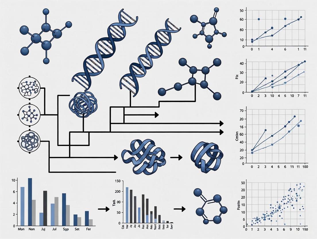
The following diagram illustrates the key conceptual relationships and decision pathways in phylogenetic signal analysis:

Phylogenetic Signal Analysis Framework

Research Applications and Future Directions

Phylogenetic signal analysis has become fundamental to diverse research applications in ecology and evolutionary biology. These include:

• Community Assembly: Understanding how phylogenetic relatedness structures ecological communities through habitat filtering or competitive exclusion [1] [2]
• Phylogenetic Niche Conservatism: Testing whether closely related species occupy similar ecological niches due to shared evolutionary constraints [1]
• Climate Change Vulnerability: Assessing whether vulnerability to climate change exhibits phylogenetic signal, allowing predictions for poorly studied species [1] [2]
• Trait Evolution: Reconstructing ancestral states and testing hypotheses about the sequence and timing of trait evolution [3]
• Drug Discovery: In pharmaceutical research, phylogenetic signal can inform the selection of model organisms and predict chemical compound distributions across plant families

The development of unified methods like the M statistic that can handle both continuous and discrete traits, as well as multiple trait combinations, represents an important advancement in the field [2]. These methods enable researchers to incorporate more comprehensive trait information and test more complex evolutionary hypotheses. As phylogenetic comparative methods continue to evolve, they will undoubtedly provide deeper insights into the patterns and processes of trait evolution across the tree of life.

The study of phylogenetic signal (PS) provides a critical window into evolutionary processes, revealing the extent to which shared ancestry explains trait variation among species. This whitepaper examines the continuum of evolutionary models, from the neutral drift described by Brownian Motion (BM) to the selective forces captured by Ornstein-Uhlenbeck (OU) and Early Burst (EB) models. BM serves as a foundational null model, characterizing trait evolution as a random walk where variance accumulates proportionally with time [5]. However, significant deviations from BM often reveal the signatures of selection. Through quantitative metrics like Pagel's λ and Blomberg's K, and their application in studies ranging from Arctic macrobenthos to Heliconius butterflies, we demonstrate how researchers can disentangle these complex evolutionary forces. This synthesis, framed within contemporary trait evolution research, offers methodological protocols and analytical frameworks essential for scientists and drug development professionals investigating the deep phylogenetic constraints and adaptive lability that shape biodiversity.

Phylogenetic Signal (PS) describes the statistical dependence between species' traits and their phylogenetic relationships, reflecting the tendency for closely related species to resemble each other more than distantly related species due to shared ancestry [6]. This phenomenon is foundational to comparative biology, as it tests the critical assumption that species are independent data points. The presence of strong PS indicates evolutionary conservatism, where traits change slowly over deep evolutionary timescales. In contrast, weak PS suggests evolutionary lability, with traits evolving rapidly, potentially due to adaptive diversification or neutral processes [6].

Quantifying PS allows researchers to move beyond descriptive patterns and infer the evolutionary processes that shape trait distributions. The measured PS is a direct outcome of the model of trait evolution a lineage has experienced. The dominant models used to explain these patterns form a continuum from purely random to deterministically selective processes, which this whitepaper explores in detail.

Brownian Motion: The Null Model of Trait Evolution

Core Properties and Mathematical Definition

Brownian Motion (BM) is a stochastic model that serves as the fundamental null hypothesis for continuous trait evolution in a phylogenetic context [5]. Originally developed to describe the random motion of particles in a fluid, BM models trait evolution as a continuous random walk where the direction and magnitude of change are uncorrelated across any time interval [5].

A BM process is mathematically defined by two parameters:

• (\bar{z}(0)): The starting value of the population mean trait at time zero.
• (\sigma^2): The evolutionary rate parameter, which determines how fast the trait value randomly wanders through trait space [5].

Under BM, the change in trait value over any time interval (t) is drawn from a normal distribution with a mean of 0 and a variance of (\sigma^2 t). This leads to three critical properties [5]:

• (E[\bar{z}(t)] = \bar{z}(0)): The expected value of the character at any time (t) is equal to its initial value, indicating no directional trend.
• Independent Increments: Changes over non-overlapping time intervals are statistically independent of one another.
• (\bar{z}(t) \sim N(\bar{z}(0),\sigma^2 t)): The trait value at time (t) is normally distributed with mean (\bar{z}(0)) and variance (\sigma^2 t).

Biological Interpretations and Implications

BM can arise from several distinct biological processes. The simplest is neutral genetic drift, where a trait, under no selective pressure, changes randomly due to the random sampling of alleles across generations [5]. However, BM can also result from selection if the direction and strength of selection fluctuate randomly through time [7]. This underscores a critical point: concluding that a trait evolves by BM does not automatically mean it is neutral; it can be consistent with a scenario of randomly changing selection [7].

Table 1: Key Properties of the Brownian Motion (BM) Model

Property	Mathematical Expression	Biological Interpretation
Expected Value	(E[\bar{z}(t)] = \bar{z}(0))	The trait shows no net directional trend over time.
Variance	(\text{Var}[\bar{z}(t)] = \sigma^2 t)	The among-lineage variance increases linearly with time.
Trait Distribution	(\bar{z}(t) \sim N(\bar{z}(0),\sigma^2 t))	Traits are normally distributed at any point in time.
Independent Evolution	Changes on distinct branches are independent.	Evolution is unconstrained and without memory of past states.

Models of Selection: Beyond the Random Walk

When trait data show significant deviations from the BM expectation, it indicates the potential action of non-random evolutionary forces. The Ornstein-Uhlenbeck and Early Burst models provide frameworks to detect and quantify these forces.

Ornstein-Uhlenbeck (OU) Model - Stabilizing Selection

The OU model extends BM by adding a parameter that simulates a central restoring force, analogous to stabilizing selection [8]. It incorporates a selective optimum (\theta) toward which the trait is pulled. The strength of this pull is determined by the parameter (\alpha) [8]. A higher (\alpha) value indicates stronger stabilizing selection, which resists deviation from the optimum and results in a bounded exploration of trait space around (\theta). This model is ideal for testing hypotheses about adaptation to specific ecological niches or functional constraints.

Early Burst (EB) Model - Adaptive Radiation

The Early Burst model, also known as the ACDC (Accelerating-Decelerating) model, describes a scenario of rapid phenotypic diversification early in a clade's history, followed by a slowdown in evolutionary rates as ecological niches become filled [6]. This pattern is a classic signature of adaptive radiation [6]. The EB model captures this by having the evolutionary rate parameter (\sigma^2) decay exponentially through time.

Comparing Evolutionary Models

The following diagram illustrates the logical relationship between evolutionary models and the processes they represent, highlighting how phylogenetic signal is used to distinguish between them.

Table 2: Comparative Analysis of Evolutionary Models for Continuous Traits

Model	Key Parameters	Evolutionary Process	Expected Phylogenetic Signal
Brownian Motion (BM)	(\bar{z}(0)), (\sigma^2)	Genetic drift or randomly changing selection [5] [7].	Variance among lineages proportional to time since divergence.
Ornstein-Uhlenbeck (OU)	(\alpha), (\theta), (\sigma^2)	Stabilizing selection toward a specific optimum trait value [8].	Trait variance is bounded; PS is strong but plateaus within selective regimes.
Early Burst (EB)	(\bar{z}(0)), (\sigma_0), (r)	Rapid initial diversification followed by slowdown (adaptive radiation) [6].	Highest trait variance among early-diverging lineages; PS depends on clade age.

Quantitative Metrics for Phylogenetic Signal

To operationalize the testing of evolutionary models, researchers rely on a suite of quantitative metrics. The table below summarizes the most widely used indices for measuring Phylogenetic Signal.

Table 3: Key Metrics for Quantifying Phylogenetic Signal

Metric	Definition	Interpretation	Value Indicating Strong PS
Pagel's λ [6]	Scales the off-diagonal elements of the variance-covariance matrix. Tests if the data fits a BM model on the tree.	λ = 0 (no PS); λ = 1 (PS fits BM expectation).	Values close to 1.0 [6].
Blomberg's K [6]	Ratio of observed PS to the PS expected under a BM model.	K > 1 indicates more PS than BM; K < 1 indicates less.	K significantly > 1.
Moran's I [6]	A spatial autocorrelation statistic adapted for phylogenies.	Positive, significant values indicate similar traits in related species.	Significant positive values [6].
Abouheif's C~mean~ [6]	Based on the autocorrelation of traits along the tips of a phylogenetic tree.	Tests for a serial independence of traits along the tree.	Significant positive values [6].

Case Studies in Decoding Evolutionary Forces

Arctic Macrobenthos Functional Traits

A comprehensive study of 50 macrobenthic species in Arctic fjords integrated mitochondrial COI-based phylogenies with 21 functional traits to investigate evolutionary constraints [6].

Experimental Protocol:

• Data Collection: Species were sampled from Kongsfjorden–Krossfjorden, Svalbard. Mitochondrial COI genes were sequenced for phylogenetic reconstruction, and 21 functional traits (e.g., tube-dwelling, burrowing, feeding mode, environmental position, reproductive traits) were coded [6].
• Phylogenetic Analysis: A phylogeny was constructed from the mtCOI sequences [6].
• Phylogenetic Signal Calculation: PS was quantified for all traits using Pagel's λ, Blomberg's K, Moran's I, and Abouheif's C~mean~ [6].
• Model Fitting: The fit of the trait data to BM, OU, and EB models of evolution was compared [6].

Key Findings:

• The majority of traits exhibited strong phylogenetic signal (Pagel's λ ≥ 1.0, p = 0.001), indicating pronounced evolutionary conservatism [6].
• Traits related to living habitat (e.g., tube-dwelling, burrowing) showed the highest autocorrelation, interpreted as adaptations to extreme Arctic conditions [6].
• Reproductive traits, in contrast, were evolutionarily labile (weak PS) [6].
• Model fitting selected the Early Burst (EB) model as the best fit for overall trait evolution, suggesting a history of rapid initial diversification [6]. Univariate analyses showed mixed patterns, with environmental position following an EB model, while body size and motility were best fit by a BM model [6].

Gene Expression inHeliconiusButterflies

A study of five Heliconius butterfly species explored the evolutionary forces acting on gene expression levels in eye and brain tissue, using BM and OU models to distinguish between drift and selection [8].

Experimental Protocol:

• RNA-seq and Orthology: RNA was extracted from the combined eye and brain tissue of biological replicates for each species. RNA-seq libraries were prepared and sequenced. Orthologous genes were grouped into orthoclusters for comparative analysis [8].
• Expression Quantification: Gene expression levels were quantified as FPKM (Fragments Per Kilobase per Million mapped reads) for each species [8].
• Model Fitting: BM and OU models were fitted to the expression data for each orthocluster using the known species phylogeny. A novel statistical test based on BM was developed to identify highly conserved genes, overcoming OU model biases in small phylogenies [8].

Key Findings:

• An estimated 81% of genes evolved under a Brownian Motion model, consistent with genetic drift [8].
• A total of 368 genes (16%) showed evidence of branch-specific shifts in expression, indicative of directional selection [8].
• Only 3% of genes were identified as highly conserved, evolving under strong stabilizing selection [8].
• The study concluded that drift is the dominant force driving gene expression evolution in these tissues, but a substantial minority of genes show signatures of selection [8].

Table 4: Key Research Reagent Solutions for Phylogenetic Comparative Studies

Reagent / Resource	Function in Research	Application Example
Mitochondrial COI Gene Markers	A standard DNA barcode region used for phylogenetic reconstruction due to its high taxonomic resolution and broad database representation [6].	Building a robust phylogeny of 50 Arctic macrobenthic species for PS analysis [6].
RNA-seq Library Prep Kits	For converting extracted RNA into sequencing-ready cDNA libraries, allowing for genome-wide expression profiling [8].	Preparing TruSeq RNA libraries from Heliconius butterfly eye and brain tissue [8].
Phylogenetic Comparative Software	Software platforms (e.g., R packages like geiger, phytools) used to calculate PS metrics and fit evolutionary models (BM, OU, EB) to trait data [6] [8].	Fitting BM, OU, and EB models to functional trait data and gene expression data [6] [8].
Functional Trait Modalities	A standardized set of defined trait states (e.g., for feeding mode, habitat position) that allow for the coding of ecological functions across diverse taxa [6].	Coding 21 distinct functional traits for Arctic macrobenthos to link phylogeny to ecosystem function [6].

The journey from detecting a phylogenetic signal to inferring the underlying evolutionary process is a cornerstone of modern comparative biology. Brownian Motion provides an essential null model, but the power of this framework lies in its ability to identify telling deviations—signatures of stabilizing selection, adaptive radiation, or directional selection. As demonstrated by empirical studies in diverse systems, from marine benthos to butterflies, the integration of robust phylogenies with quantitative trait data and powerful model-fitting statistics allows researchers to move beyond pattern description to process inference. This methodological pipeline, supported by the detailed protocols and resources outlined in this whitepaper, is critical for accurately interpreting the evolutionary history of traits, with profound implications for predicting evolutionary responses to environmental change and even for informing drug discovery by understanding the evolution of molecular pathways.

Phylogenetic signal (PS) quantifies the tendency for related species to resemble each other more than distant relatives, a cornerstone concept for interpreting trait evolution. This technical guide elucidates the core principles, measurement methodologies, and diverse applications of PS across ecological, evolutionary, and medical disciplines. We synthesize current research to provide a comprehensive framework for analyzing evolutionary constraints, from deep phylogenetic conservatism to adaptive lability. The document includes standardized protocols for quantifying PS, detailed workflows for evolutionary model selection, and a curated toolkit of research reagents, equipping scientists with the necessary resources to integrate phylogenetic comparative methods into their research programs.

Phylogenetic signal (PS) describes the statistical dependence between species' traits and their phylogenetic relationships, reflecting the pattern where closely related species often exhibit more similar phenotypes than those drawn at random from the same tree [6]. This phenomenon is fundamentally linked to evolutionary niche conservatism, the tendency of species to retain ancestral ecological characteristics [6]. The presence and strength of PS indicate the extent to which trait evolution is constrained by shared ancestry, providing critical insights into the processes shaping biodiversity, from adaptive radiation to phylogenetic inertia.

The measurement and interpretation of PS are foundational to modern comparative biology. In an era of rapid environmental change, understanding phylogenetic constraints is vital for predicting species responses to anthropogenic pressures, identifying conserved functional traits in drug discovery, and reconstructing pathogen emergence dynamics. This guide establishes a unified framework for PS analysis, bridging conceptual foundations with practical applications across diverse research domains.

Quantifying Phylogenetic Signal: Metrics and Models

Accurate quantification of PS requires multiple complementary approaches, each with distinct statistical properties and evolutionary assumptions. The table below summarizes the primary metrics used in contemporary research.

Table 1: Key Metrics for Quantifying Phylogenetic Signal

Metric	Statistical Basis	Interpretation	Optimal Use Cases
Pagel's λ [6]	Brownian Motion model transformation (0-1)	λ=1: Strong signal; λ=0: No signal	Testing evolutionary hypotheses under Brownian motion; general-purpose signal detection
Blomberg's K [6]	Variance ratio among clades vs. tip randomisation	K>1: Stronger signal than BM; K<1: Weaker signal	Comparing signal strength across traits and trees; assessing trait lability
Moran's I [6]	Spatial autocorrelation applied to phylogeny	I>0: Positive autocorrelation; I<0: Negative autocorrelation	Detecting phylogenetic clustering at different evolutionary depths
Abouheif's C~mean~ [6]	Autocorrelation along phylogenetic adjacency	C>0: Similar traits in adjacent lineages	Identifying local phylogenetic constraints and adaptive shifts

These metrics operate within a broader framework of evolutionary models that test specific hypotheses about trait evolution:

• Brownian Motion (BM): Models random trait drift where variance accumulates proportionally with time [6] [9].
• Ornstein-Uhlenbeck (OU): Incorporates stabilizing selection toward a selective optimum [6].
• Early Burst (EB): Describes rapid initial diversification followed by evolutionary deceleration [6].

Model selection criteria (e.g., AICc) determine which evolutionary process best explains observed trait distributions, providing mechanistic insights beyond signal detection alone.

Applications in Ecology and Evolution

Case Study: Functional Trait Evolution in Arctic Macrobenthos

Research on macrobenthic communities in Svalbard fjords demonstrates PS analysis in extreme environments. Integrating mitochondrial cytochrome c oxidase subunit I (mtCOI)-based phylogenies with 21 functional traits for 50 species revealed a hierarchy of evolutionary constraints [6] [10].

Table 2: Phylogenetic Signal Strength Across Macrobenthic Functional Traits

Trait Category	Specific Traits	Signal Strength	Evolutionary Interpretation
Living Habitat	Tube-dwelling, Burrowing	Strong (C~mean~=0.310, p=0.002) [6]	Pronounced conservatism; adaptation to extreme Arctic conditions
Feeding Habits	Feeding mechanisms, Trophic level	Intermediate	Moderate phylogenetic constraint with ecological flexibility
Environmental Position	Sediment positioning, Mobility	Strong (Pagel's λ≥1.0, p=0.001) [6]	Deep phylogenetic constraints on habitat use
Reproductive Strategies	Fecundity, Larval development	Labile (Weak PS)	High evolutionary flexibility in response to selective pressures

The evolutionary model fitting identified Early Burst as the best model for overall trait evolution, suggesting rapid initial diversification followed by evolutionary deceleration in these communities [6]. This hierarchical constraint structure, where habitat traits show strong conservatism while reproductive traits remain labile, illustrates how PS analysis deciphers complex evolutionary histories in natural systems.

Phylogenetic Signal in Species Distribution Models

PS analysis critically informs predictive ecology by revealing discrepancies between biogeographic predictions and empirical observations. A study of three Acer species cultivated in UK botanic gardens found that conventional Species Distribution Models (SDMs) based on niche overlap failed to predict survival rates accurately [11]. While A. davidii showed high habitat suitability predictions, it exhibited the lowest survival; conversely, A. pictum demonstrated high survival despite model predictions of unsuitability [11]. The observed phylogenetic signal in survival patterns indicated that intrinsic traits related to climate tolerance, conserved yet masked in conventional modeling approaches, better explained performance outcomes [11]. This highlights the necessity of incorporating phylogenetic information to bridge the gap between macro-scale predictions and local-scale individual performance.

Medical and Pharmaceutical Applications

Pathogen Evolution and Outbreak Surveillance

Phylogenetic signal analysis forms the backbone of modern pathogen genomics and epidemic response. During the 2025 Kasai Ebola virus (EBOV) outbreak, phylogenetic reconstruction of four genomes enabled critical assessments of transmission dynamics and temporal origins [12]. Researchers identified phylogenetically incompatible mutations suggesting homoplasy, reversion, or sequencing errors, which required masking to avoid distorting phylogenetic and temporal signal [12]. Time-scaled phylogenetic analysis using BEAST software estimated the time to most recent common ancestor (tMRCA), helping determine whether the outbreak significantly pre-dated first detection [12]. This application demonstrates how phylogenetic signal in pathogen genomes directly informs public health interventions and outbreak containment strategies.

Phylogenetic Conservation in Drug Discovery

Evolutionary conservation analysis identifies potential therapeutic targets through detecting phylogenetic signal in functionally important biomolecules. The SatuTe algorithm exemplifies advanced approaches to quantifying phylogenetic information in molecular data, identifying which branches in a tree and which alignment regions maintain strong phylogenetic signal despite saturation effects [13]. This methodology is particularly valuable for distinguishing well-supported phylogenetic relationships from those with diminished signal, with direct implications for identifying conserved functional domains in drug target discovery [13].

Furthermore, microbial phylogenomics benefits from tailored marker gene selection using tools like TMarSel, which systematically selects gene families beyond standard universal orthologs to improve phylogenetic accuracy [14]. This approach identifies markers with functional annotations beyond traditional housekeeping genes, including metabolism, cellular processes, and environmental information processing [14], expanding the potential targets for antimicrobial drug development.

Experimental Protocols and Methodologies

Standard Workflow for Phylogenetic Signal Analysis

The following protocol outlines a comprehensive approach for analyzing phylogenetic signal in trait data, synthesizing methodologies from cited studies.

Advanced Protocol: Testing Evolutionary Models

For researchers investigating specific evolutionary processes, the following detailed protocol implements model-based approaches:

• Data Requirements: Time-calibrated phylogeny with branch lengths; continuous or discrete trait measurements for all tips; appropriate data transformation if needed.
• Model Specification:
  • Brownian Motion (BM): Single parameter (σ²) describing evolutionary rate.
  • Ornstein-Uhlenbeck (OU): Three parameters (σ², α, θ) modeling selection strength and optimum.
  • Early Burst (EB): Parameters (σ², r) capturing exponential decrease in evolutionary rate.
• Computational Implementation:
  • Use R packages (phytools, geiger, ape) or specialized software (BEAST, RevBayes).
  • Apply maximum likelihood or Bayesian inference for parameter estimation.
  • Compare models using AICc, AICw, or Bayes factors.
• Model Diagnostics:
  • Check for adequate model fit using phylogenetic residuals.
  • Test for among-lineage rate variation.
• Sensitivity Analysis:
  • Assess robustness to phylogenetic uncertainty using tree blocks or posterior distributions.
  • Apply robust regression methods to mitigate effects of tree misspecification [9].

Mitigating Tree Misspecification with Robust Methods

Comparative studies are highly sensitive to phylogenetic accuracy. Recent simulations demonstrate that conventional phylogenetic regression yields excessively high false positive rates when incorrect trees are assumed, with worsening performance as dataset size increases [9]. Robust sandwich estimators substantially reduce this sensitivity, effectively rescuing phylogenetic analyses under realistic conditions of tree misspecification [9]. This approach is particularly valuable for large-scale genomic studies where gene tree-species tree discordance is prevalent.

The Scientist's Toolkit: Essential Research Reagents

The table below catalogs critical methodological tools for phylogenetic signal analysis, drawn from current research applications.

Table 3: Essential Reagents and Software for Phylogenetic Signal Research

Tool Name	Type/Category	Primary Function	Application Context
mtCOI gene [6]	Molecular marker	Species identification & phylogenetics	Macrobenthic community phylogenies
Pagel's λ & Blomberg's K [6]	Statistical metrics	Quantify phylogenetic signal	General trait evolution analysis
ASTRAL-Pro2 [14]	Software algorithm	Species tree from gene trees	Handling gene tree discordance
SatuTe [13]	Analysis tool	Measure phylogenetic information	Identifying saturated alignment regions
TMarSel [14]	Selection algorithm	Tailored marker gene selection	Microbial phylogenomics with MAGs
Robust Phylogenetic Regression [9]	Statistical method	Mitigate tree misspecification effects	Large-scale comparative analyses
BEAST [12]	Software platform	Bayesian evolutionary analysis	Pathogen molecular dating
PrimConsTree [15]	Consensus algorithm	Tree synthesis with branch lengths	Integrating phylogenetic uncertainty

Phylogenetic signal analysis provides an essential framework for interpreting trait evolution across biological disciplines. From understanding functional trait constraints in Arctic benthos to tracking pathogen emergence and identifying conserved drug targets, PS quantification bridges evolutionary history with contemporary function. The methodologies outlined in this guide—from standardized metrics and evolutionary models to robust statistical approaches—equip researchers with tools to decode evolutionary patterns in an increasingly complex biological world. As genomic and trait datasets expand, integrating phylogenetic signal analysis will remain fundamental for predicting biological responses to environmental change and advancing biomedical discovery.

Phylogenetic Niche Conservatism and the Conservation of Traits Over Time

Phylogenetic Niche Conservatism (PNC) is a central concept in evolutionary biology describing the tendency of species to retain ancestral ecological characteristics over evolutionary time. It represents the phylogenetic signal in ecological traits, where closely related species exhibit more similar niche requirements than would be expected by random chance alone. This phenomenon plays a fundamental role in shaping biogeographic patterns, species distributions, and biodiversity dynamics. Understanding PNC provides crucial insights for predicting responses to environmental change, elucidating biogeographic history, and formulating effective biodiversity conservation strategies [16] [17].

The significance of PNC extends across multiple disciplines. For ecological and evolutionary research, it helps explain large-scale biodiversity patterns, including the latitudinal diversity gradient where tropical regions harbor higher species richness. For conservation science, identifying PNC allows prioritization of species and populations that may be most vulnerable to climate change due to their limited adaptive potential. For drug development professionals, understanding conserved traits across plant lineages can inform the search for novel bioactive compounds in related species [16] [18].

Empirical Evidence and Case Studies

Evidence from Floristic Studies

Recent studies across diverse plant taxa provide compelling evidence for widespread phylogenetic niche conservatism. Research on Chinese woody endemic flora, encompassing 1,370 species, revealed moderate to high phylogenetic signals in key functional traits including leaf length, maximum height, and seed diameter. This trait conservation indicates evolutionary constraints that potentially impact adaptability to climate change. The study further uncovered a phylogenetically conserved coordination between plant height and leaf length that operated independently of macroecological patterns of temperature and precipitation, emphasizing the fundamental role of phylogenetic ancestry in shaping endemic species distribution [19].

Niche Evolution in Relictual Gymnosperms

Comprehensive analysis of Taxus (yew) lineages demonstrates the complex interplay between niche conservatism and divergence. As a Tertiary relict gymnosperm with 11 lineages distributed across East Asia, Taxus provides an excellent model for studying montane species' niche evolution. Research integrating ensemble ecological niche models with phylogenetic reconstruction identified both niche conservatism and divergence patterns, with early conservatism followed by recent divergence. Key environmental variables including extreme temperature, temperature and precipitation variability, light, and altitude were identified as major drivers of current niche divergence among lineages [16].

The Taxus study classified eleven lineages into four distinct clades with characteristic niche properties. The Northern clade (T. cuspidata) and Central clade (T. chinensis, T. qinlingensis, and the Emei type) retained ancestral drought and cold tolerance, displaying significant PNC. In contrast, the Southern clade (T. calcicola, T. phytonii, T. mairei, and the Huangshan type) exhibited high heat and moisture tolerance, suggesting an adaptive shift. Orogenic activities and climate changes in the Tibetan Plateau since the Late Miocene likely facilitated local adaptation of ancestral populations, driving their expansion and diversification [16].

Tropical Niche Conservatism Hypothesis

The Tropical Niche Conservatism Hypothesis (TNCH) was tested using the genus Escallonia in South America, integrating phylogeny, paleoclimate estimation, and current niche modeling. Contrary to some predictions of TNCH, Escallonia originated in the early Eocene (52.17 ± 0.85 My) under microthermal to mesothermal climates (mean annual temperature of 13.8°C), not megathermal conditions. The evolutionary models predominantly followed Brownian motion and Ornstein-Uhlenbeck processes, with phylogenetic signals detected in 7 of 9 climate variables, indicating significant climatic niche conservatism. The study demonstrated how Escallonia, originating in the central and southern Andes, reached other environments through dispersal while largely conserving its ancestral niche [18].

Table 1: Key Case Studies Demonstrating Phylogenetic Niche Conservatism

Study System	Taxonomic Group	Key Conserved Traits	Evolutionary Models Identified	Reference
Chinese Woody Endemics	Woody plants	Leaf length, maximum height, seed diameter	Not specified	[19]
East Asian Yews (Taxus)	Gymnosperms	Drought and cold tolerance (Northern & Central clades)	Early conservatism, recent divergence	[16]
Escallonia	Angiosperms	Temperature-related variables (7 of 9 climate variables)	Brownian motion, Ornstein-Uhlenbeck	[18]
Dipterocarpaceae	Tropical trees	Height, diameter, shade tolerance	Phylogenetic signal (moderate to strong)	[17]

Methodological Framework

Phylogenetic Comparative Methods

The investigation of PNC relies heavily on phylogenetic comparative methods (PCMs) that statistically account for non-independence of species due to shared evolutionary history. These methods enable researchers to test whether ecological traits exhibit phylogenetic signal, measure the strength of this signal, and infer evolutionary processes that have shaped trait distributions across phylogenies [20].

A fundamental approach in PCMs is the use of evolutionary models to describe how traits change over time. The Brownian motion (BM) model represents random trait evolution analogous to a random walk, serving as a null model. The Ornstein-Uhlenbeck (OU) model incorporates stabilizing selection around an optimal trait value. Early-Burst (EB) models describe rapid initial diversification that slows over time. More complex models allow for shifts in evolutionary parameters across the phylogeny [20].

Phylogenetic Independent Contrasts

Phylogenetic Independent Contrasts (PICs), introduced by Felsenstein (1985), provide a method to estimate rates of evolutionary change while accounting for phylogenetic relationships. The method calculates standardized contrasts between sister taxa or nodes, representing independent evolutionary comparisons [21].

The PIC algorithm involves:

• Identifying adjacent tips on the phylogeny with a common ancestor
• Computing raw contrasts as the difference between their trait values: ( c{ij} = xi - x_j )
• Standardizing contrasts by their expected variance: ( s{ij} = \frac{c{ij}}{vi + vj} )

These standardized contrasts are both independent and identically distributed under a Brownian motion model, allowing statistical analyses without phylogenetic non-independence [21].

Advanced Analytical Approaches

Recent methodological advances include Evolutionary Discriminant Analysis (EvoDA), which applies supervised learning to predict evolutionary models via discriminant analysis. This approach offers potential improvements over conventional model selection, particularly for traits subject to measurement error, which reflects realistic conditions in empirical datasets [20].

Phyloclimatic modeling represents another advanced framework, integrating ecological niche models with phylogenetic data to reconstruct ancestral niche breadth, ecological tolerances, and niche trait disparity over time. This approach has been applied to diverse taxa including Scutiger boulengeri, Viperidae, and Abies to study niche evolution [16].

Table 2: Methodological Approaches for Studying Phylogenetic Niche Conservatism

Method Category	Specific Techniques	Primary Applications	Considerations
Evolutionary Models	Brownian motion, Ornstein-Uhlenbeck, Early-Burst	Modeling trait evolution processes	Different models imply different evolutionary processes
Phylogenetic Signal Tests	Pagel's lambda, Blomberg's K, Moran's I	Quantifying trait phylogenetic dependence	Varying statistical power and interpretation
Comparative Methods	Phylogenetic Independent Contrasts, PGLS	Accounting for phylogenetic non-independence	Assumptions about evolutionary model
Integrated Approaches	Phyloclimatic modeling, Ensemble ENMs	Reconstructing niche evolution	Combines occurrence, environmental, and phylogenetic data
Machine Learning	Evolutionary Discriminant Analysis	Model selection with noisy data	Emerging approach, requires validation

Experimental Protocols and Research Workflows

Integrated Phyloclimatic Analysis

A comprehensive protocol for investigating PNC involves multiple integrated steps:

• Data Collection

  • Gather species occurrence records from herbarium specimens, field surveys, and biodiversity databases
  • Obtain environmental data layers (temperature, precipitation, altitude, soil characteristics)
  • Sequence molecular markers (chloroplast DNA, ITS, nuclear genes) for phylogenetic reconstruction

• Phylogenetic Reconstruction

  • Align DNA sequences using appropriate algorithms
  • Reconstruct phylogenetic relationships using Bayesian inference or maximum likelihood methods
  • Estimate divergence times with fossil calibrations or molecular clock approaches

• Niche Modeling

  • Develop ensemble ecological niche models (eENMs) using multiple algorithms
  • Project models to current and paleoclimatic scenarios
  • Evaluate model performance with cross-validation techniques

• Niche Similarity Analysis

  • Conduct environmental PCA (PCA-env) to visualize niche overlap in multivariate space
  • Perform niche identity and background tests to assess niche equivalency and similarity
  • Quantify niche overlap using Schoener's D or related metrics

• Phyloclimatic Modeling

  • Reconstruct ancestral niche characteristics using comparative methods
  • Test for phylogenetic signal in climatic variables using Pagel's λ or Blomberg's K
  • Fit alternative evolutionary models (BM, OU, EB) to niche-related traits

This integrated approach was successfully applied in Taxus research, revealing how orogenic activities and climate changes in the Tibetan Plateau since the Late Miocene facilitated local adaptation and diversification [16].

Trait-Based Conservation Prioritization

For conservation applications, the following protocol identifies priority species based on PNC:

• Phylogenetic Signal Quantification

  • Measure phylogenetic signal in functional traits using Pagel's λ or Blomberg's K
  • Test for phylogenetic conservatism in climatic tolerances

• PNC Level Assessment

  • Compare observed trait distributions across phylogeny to null models
  • Rank species according to their degree of phylogenetic niche conservatism

• Vulnerability Evaluation

  • Project future climate change scenarios for species distributions
  • Identify species with high PNC in threatened habitats

• Conservation Prioritization

  • Prioritize species exhibiting highest PNC levels for conservation efforts
  • Focus protection on geographic regions containing multiple PNC species

This approach recommended prioritizing T. qinlingensis conservation due to its high PNC level, particularly in the Qinling, Daba, and Taihang Mountains, where populations are highly degraded and vulnerable to future climate fluctuations [16].

Research Tools and Reagents

Table 3: Essential Research Toolkit for Phylogenetic Niche Conservatism Studies

Category	Specific Tools/Reagents	Function/Application	Examples from Literature
Molecular Markers	Chloroplast DNA sequences (cpDNA), Internal Transcribed Spacer (ITS), Nuclear genes (NEEDLY)	Phylogenetic reconstruction and divergence time estimation	13 cpDNA regions, ITS, and NEEDLY used for Taxus phylogeny [16]
Software Packages	Bayesian inference programs, Ecological Niche Modeling platforms, R packages for comparative methods	Data analysis and model fitting	Bayesian trees, ensemble ENMs, phyloclimatic modeling [16] [20]
Environmental Data	WorldClim, Paleoclimate databases, Soil maps, Altitude layers	Characterizing ecological niches	Historical climate reconstructions for Escallonia [18]
Statistical Frameworks	Brownian motion, Ornstein-Uhlenbeck, Early-Burst models	Modeling trait evolution	BM and OU as predominant models in Escallonia [18]
Experimental Approaches	Phylogenetic Independent Contrasts, Evolutionary Discriminant Analysis	Accounting for phylogeny in comparative analyses	Independent contrasts for evolutionary rate estimation [21] [20]

Implications for Conservation and Drug Development

Biodiversity Conservation Strategies

The demonstration of phylogenetic niche conservatism has profound implications for biodiversity conservation. Simulation studies have revealed that niche conservatism promotes biological diversification, whereas labile niches generally lead to slower diversification rates. These findings result from elevated speciation rates under niche conservatism scenarios, where species' inability to adapt to new conditions causes range fragmentation, population isolation, and subsequent allopatric speciation [22].

Conservation strategies must consider the consequences of PNC for long-term population changes. Research on Dipterocarpaceae, keystone plants in Southeast Asian tropical forests, found that conservation status is related to phylogeny and correlated with population trend status. This phylogenetic dependency of extinction risk necessitates conservation approaches that incorporate evolutionary history [17].

For endemic species with limited ranges, PNC presents particular challenges. Chinese woody endemic flora showed evolutionary constraints in functional traits that potentially impact adaptability to climate change. This suggests that range-limited endemics may require prioritized in-situ conservation and carefully designed ex situ conservation strategies [19].

Drug Discovery Applications

For drug development professionals, understanding PNC provides valuable insights for bioprospecting strategies. The non-random phylogenetic distribution of ecological traits extends to biochemical characteristics, including the production of secondary metabolites with medicinal properties. The conservation of paclitaxel (a widely used anti-cancer drug) across Taxus lineages demonstrates how phylogenetic information can guide the search for novel bioactive compounds [16].

The integration of phylogenetic approaches with drug discovery offers a powerful framework for:

• Identifying novel sources of known bioactive compounds by examining closely related species
• Predicting chemical diversity across plant lineages based on phylogenetic relationships
• Prioritizing species for biochemical screening using phylogenetic information
• Understanding evolutionary patterns of medically relevant traits

Visualizing Concepts and Relationships

Core Concept of Phylogenetic Niche Conservatism

Methodological Workflow for PNC Research

Phylogenetic niche conservatism represents a fundamental pattern in evolutionary biology with far-reaching implications for understanding biodiversity patterns, predicting responses to environmental change, and guiding conservation efforts. The integration of phylogenetic comparative methods with ecological niche modeling has revealed how conserved ecological traits influence diversification dynamics across disparate lineages and ecosystems.

The empirical evidence from diverse systems—including Chinese woody endemics, East Asian yews, Escallonia, and dipterocarps—consistently demonstrates the prevalence of phylogenetic signal in ecological traits. Methodological advances continue to enhance our ability to detect and quantify PNC, from traditional phylogenetic independent contrasts to emerging machine learning approaches like Evolutionary Discriminant Analysis.

For conservation practitioners and drug development professionals, incorporating phylogenetic niche conservatism into research frameworks provides valuable insights for prioritizing conservation efforts and guiding bioprospecting strategies. As climate change accelerates, understanding the constraints imposed by phylogenetic history on ecological adaptability becomes increasingly crucial for effective biodiversity management and sustainable resource utilization.

The Researcher's Toolkit: Quantifying Signals and Powering Drug Discovery

Phylogenetic signal quantifies the tendency for related species to resemble each other more than they resemble species drawn at random from a phylogenetic tree, representing a cornerstone concept in modern evolutionary biology [23]. Accurate measurement of phylogenetic signal is methodologically crucial for selecting appropriate comparative methods and substantively important for inferring broad-scale evolutionary and ecological processes, such as phylogenetic niche conservatism [24] [23]. This technical guide provides an in-depth examination of four principal metrics—Blomberg's K, Pagel's λ, Moran's I, and the D statistic—framed within contemporary trait evolution research. We present structured comparisons, detailed experimental protocols, and practical toolkits to equip researchers and drug development professionals with robust analytical frameworks for evolutionary inference, addressing both theoretical foundations and application challenges in comparative phylogenetics.

The foundational principle of phylogenetic signal stems from the recognition that species share evolutionary histories, creating statistical non-independence that must be accounted for in comparative analyses [23]. Phylogenetic signal is formally defined as "a tendency for related species to resemble each other more than they resemble species drawn at random from a tree" [23]. This concept transcends mere methodological correction, offering fundamental insights into evolutionary processes including adaptive radiation, stabilizing selection, and phylogenetic niche conservatism.

Modern comparative methods require careful quantification of phylogenetic signal to determine whether phylogenetic corrections are necessary and to test evolutionary hypotheses [24]. The metrics discussed herein—K, λ, I, and D—operate under different statistical philosophies and assumptions, making them suitable for distinct research contexts. Model-based approaches (K and λ) explicitly contrast trait data against evolutionary models (typically Brownian motion), while statistical approaches (I and related methods) quantify autocorrelation without strong evolutionary model assumptions [24] [23].

Understanding these metrics' properties, strengths, and limitations enables researchers to select optimal tools for diverse applications, from traditional trait evolution studies to emerging fields like comparative oncology [25], where phylogenetic patterns in disease susceptibility across species inform human health vulnerabilities.

Theoretical Foundations and Metric Comparisons

Evolutionary Models as a Framework

Most phylogenetic signal metrics reference explicit evolutionary models, with Brownian motion serving as the primary null hypothesis [25]. Under Brownian motion, phenotypic divergence among species increases linearly with time, resulting from either neutral genetic drift or random responses to environmental fluctuations [23]. The expected covariance between species under Brownian motion equals their shared evolutionary branch length [25].

Extensions to Brownian motion provide more complex evolutionary scenarios:

• Ornstein-Uhlenbeck (OU) model: Incorporates a stabilizing selection component that pulls traits toward an optimum [25]
• Mean trend model: Adds directional drift to Brownian motion [25]
• Rate trend model: Allows evolutionary rates to change over time [25]

These models establish expectations against which observed trait distributions can be compared to quantify phylogenetic signal.

Comparative Table of Key Metrics

Table 1: Core characteristics of major phylogenetic signal metrics

Metric	Theoretical Basis	Value Interpretation	Strengths	Common Applications
Blomberg's K [26]	Variance ratio compared to Brownian motion expectation	K = 1: Brownian motion; K < 1: less signal than BM; K > 1: more signal than BM	Clear biological interpretation; Handles large datasets	Testing evolutionary model fit; Trait lability assessment
Pagel's λ [26] [25]	Branch-length transformation of phylogenetic correlations	0-1 range (theoretical); λ=0: no signal; λ=1: Brownian motion	Natural scale; Integrated with likelihood framework	Phylogenetic generalized least squares; Model comparison
Moran's I [23]	Spatial autocorrelation adapted for phylogeny	I > 0: positive autocorrelation; I < 0: negative autocorrelation	No detailed phylogeny required; Flexible weighting matrices	Initial signal screening; Incomplete phylogenetic information
D Statistic [27]	Binary trait evolution model	D = 0: Brownian motion; D = 1: random distribution	Specialized for binary traits; Explicit evolutionary model	Presence/absence traits; Disease trait evolution

Table 2: Statistical properties and data requirements

Metric	Data Type	Phylogeny Requirement	Statistical Test	Implementation
Blomberg's K	Continuous	Ultrametric preferred	Randomization or permutation	R: phylosig() in phytools
Pagel's λ	Continuous	Ultrametric	Likelihood ratio test	R: phylosig(method="lambda")
Moran's I	Continuous or discrete	Distance matrix sufficient	Approximation to normal distribution	R: Moran.I() in ape
D Statistic	Binary	Ultrametric	Comparison to simulated distributions	R: phylo.d() in caper

Key Differences and Practical Implications

While all metrics quantify phylogenetic signal, they operationalize this concept differently. Pagel's λ measures the similarity of trait covariances to Brownian motion expectations by scaling internal branch lengths [26] [25], whereas Blomberg's K represents a variance partitioning ratio [26]. This fundamental difference means they may yield divergent conclusions for the same dataset [26]. For example, a trait might show K < 1 (suggesting less phylogenetic structure than Brownian motion) while λ ≈ 1 (indicating strong phylogenetic covariance structure).

Moran's I offers distinct advantages when detailed phylogenies are unavailable or when trait evolution deviates significantly from standard models [24] [23]. Statistical approaches based on autocorrelation remain particularly valuable for non-standard evolutionary scenarios or when phylogenetic information is incomplete.

Detailed Methodological Protocols

Workflow for Phylogenetic Signal Analysis

Diagram 1: Phylogenetic signal analysis workflow

Estimating Blomberg's K

Theoretical Basis: Blomberg's K compares the observed variance among sister clades to the variance expected under Brownian motion evolution [26]. The metric is calculated as a ratio of the mean squared error (MSE) of tip data under a Brownian motion model to the MSE of phylogenetic independent contrasts [26].

Protocol:

• Data Preparation: Compile continuous trait measurements for each species and an ultrametric phylogenetic tree
• Calculation:
  • Compute the mean squared error of the tip data under Brownian motion (MSE₀)
  • Calculate the mean squared error of the phylogenetic independent contrasts (MSE)
  • Determine the expected value of MSE/MSE₀ under Brownian motion
• Statistical Testing:
  • Perform randomization tests by shuffling trait values across tips
  • Generate null distribution of K values under no phylogenetic signal
  • Compare observed K to null distribution for p-value calculation
• Interpretation:
  • K ≈ 1: Evolution consistent with Brownian motion
  • K < 1: Phylogenetic signal weaker than Brownian motion (traits more labile)
  • K > 1: Stronger phylogenetic signal than Brownian motion (traits more conserved)

Estimating Pagel's λ

Theoretical Basis: Pagel's λ transforms internal branch lengths of the phylogenetic tree by multiplying them by λ, effectively scaling the phylogenetic covariance matrix [25]. The maximum likelihood estimate of λ indicates the strength of phylogenetic signal.

Protocol:

• Data Preparation: Assemble continuous trait data and ultrametric phylogeny
• Likelihood Optimization:
  • Compute log-likelihood for trait data under Brownian motion model
  • Iteratively optimize λ value (0 ≤ λ ≤ 1) that maximizes likelihood
  • Transform tree using optimized λ parameter
• Hypothesis Testing:
  • Compare likelihood of estimated λ to models where λ = 0 (no signal)
  • Perform likelihood ratio test: LR = -2 × (logLik₀ - logLik₁)
  • Assess significance using χ² distribution with 1 degree of freedom
• Interpretation:
  • λ = 0: No phylogenetic signal (traits evolve independently)
  • λ = 1: Strong phylogenetic signal (Brownian motion evolution)
  • 0 < λ < 1: Intermediate phylogenetic signal

Estimating Moran's I

Theoretical Basis: Moran's I measures spatial autocorrelation adapted for phylogenetic relationships by quantifying similarity between species as a function of their phylogenetic proximity [23].

Protocol:

• Matrix Construction:
  • Create phylogenetic distance matrix (D) from tree
  • Convert to weighting matrix (W) using inverse distance or binary thresholds
  • Standardize weighting matrix to row sums of unity
• Calculation:
  • Compute global Moran's I using formula: I = (n/S₀) × [ΣᵢΣⱼ wᵢⱼ(yᵢ - ȳ)(yⱼ - ȳ)] / [Σᵢ(yᵢ - ȳ)²] where n is number of species, wᵢⱼ are weights, yᵢ and yⱼ are trait values, ȳ is mean trait value, and S₀ = ΣᵢΣⱼ wᵢⱼ
• Significance Testing:
  • Calculate expected I under null hypothesis of no autocorrelation
  • Derive standard error using matrix permutations
  • Compute z-score: z = (I - E[I]) / SE[I]
• Interpretation:
  • I > E[I]: Positive phylogenetic autocorrelation (signal present)
  • I < E[I]: Negative phylogenetic autocorrelation (overdispersion)
  • I ≈ E[I]: No phylogenetic signal

Case Study: Phylogenetic Signal in Ecotoxicology

Background: Species Sensitivity Distributions (SSDs) in ecotoxicology traditionally assume data points are independent and identically distributed, ignoring potential phylogenetic non-independence [27].

Experimental Approach:

• Compiled toxicity data for aquatic autotrophs exposed to atrazine and aquatic/avian species exposed to chlorpyrifos [27]
• Constructed phylogenetic trees using taxonomic identifiers from NCBI and phyloT generator [27]
• Generated phylogenetic distance matrices using cophenetic function in R 'ape' package [27]
• Tested for phylogenetic signal in toxicity endpoints using multiple metrics
• Compared SSDs and hazardous concentrations (HC5 values) with and without accounting for phylogeny

Findings: Significant phylogenetic signal occurred in several chlorpyrifos datasets but not in atrazine datasets [27]. When present, phylogenetic signal reduced effective sample size but had minimal impact on HC5 values, demonstrating SSDs' robustness to violations of independence assumptions [27].

Critical Considerations in Application

Metric Selection and Interpretation

Diagram 2: Metric selection decision framework

Methodological Challenges and Robust Solutions

Tree Sensitivity: Phylogenetic signal estimates demonstrate concerning sensitivity to phylogenetic tree choice [9]. Recent simulations reveal that false positive rates in phylogenetic regression can approach 100% with incorrect tree specification, particularly as dataset size increases [9]. Robust regression techniques employing sandwich estimators can mitigate these effects, maintaining acceptable false positive rates even under tree misspecification [9].

Taxonomic Sampling: Pagel's λ exhibits particular sensitivity to taxonomic sampling completeness. The addition of sister taxa can dramatically increase λ estimates without changes to the underlying evolutionary process, as the metric treats tip branches differently from internal branches [28]. This biological nonsensical property necessitates careful interpretation, particularly in incompletely sampled clades.

Timescale Considerations: Traditional metrics like K and λ conceptualize phylogenetic signal as uniform across timescales, while biological reality often involves signal degradation over deeper divergences [28]. The Ornstein-Uhlenbeck α parameter provides a theoretically superior alternative for modeling timescale-dependent signal decay, with units (1/time) that offer biologically meaningful interpretation [28].

Emerging Applications in Evolutionary Medicine

Comparative oncology exemplifies how phylogenetic signal analyses illuminate disease patterns across species [25]. Cancer risk variation across mammals displays significant phylogenetic signal, reflecting shared evolutionary constraints on somatic maintenance mechanisms [25]. These analyses reveal how life history trade-offs between reproduction and DNA repair evolve along phylogenetic lineages, informing understanding of human cancer vulnerabilities within a broader evolutionary context [25].

Research Toolkit

Table 3: Key software and implementation resources

Tool/Platform	Primary Function	Key Functions	Access
R with ape package [27]	Phylogenetic analysis	cophenetic(), Moran.I()	CRAN
R with phytools package [26]	Phylogenetic comparative methods	phylosig() for K and λ	CRAN
phyloT generator [27]	Phylogenetic tree construction	Generate trees from taxonomic IDs	Online tool
NCBI Taxonomy Database [27]	Taxonomic reference	Standardized species identifiers	Public database

Experimental Reagents and Materials

Table 4: Essential resources for empirical phylogenetic signal studies

Resource Type	Specific Examples	Application Context	Critical Considerations
Trait Datasets	Species toxicity endpoints [27], Life history traits [9], Gene expression data [25]	Various comparative analyses	Data quality, standardization, phylogenetic scale
Phylogenetic Trees	Time-calibrated supertrees [23], Gene trees [9], Species trees [9]	Evolutionary model fitting	Branch length accuracy, taxonomic coverage
Statistical Packages	R, PDAP, custom simulation scripts [26] [23]	Metric calculation, significance testing	Method assumptions, computational efficiency

Accurate quantification of phylogenetic signal represents a fundamental step in evolutionary research, informing both methodological approaches and biological interpretation. Blomberg's K, Pagel's λ, Moran's I, and the D statistic offer complementary perspectives on the pattern of trait evolution across phylogenies, each with distinct strengths, limitations, and appropriate application contexts. As comparative datasets expand in size and complexity, particularly in emerging fields like evolutionary medicine, robust phylogenetic signal assessment becomes increasingly crucial for valid biological inference. Researchers must carefully select metrics based on their specific data structures, phylogenetic information, and biological questions, while remaining mindful of methodological challenges including tree sensitivity and taxonomic sampling effects. Future methodological developments will likely focus on more nuanced models of trait evolution that better capture the complexity of phylogenetic signal across timescales and biological levels.

The study of phylogenetic signals—the tendency for related species to resemble each other more than distant relatives—is a cornerstone of ecological and evolutionary research [2]. Accurate detection of these signals is crucial for understanding trait evolution, community assembly, and species' responses to environmental change. However, existing methods face significant limitations: they are typically designed for either continuous or discrete traits, and they struggle with multiple trait combinations despite biological functions often arising from trait interactions [2]. This whitepaper introduces the M statistic, a unified methodological framework for detecting phylogenetic signals across continuous traits, discrete traits, and multiple trait combinations. We present a comprehensive technical guide detailing the method's theoretical foundation, experimental validation, and practical implementation, positioning it as an essential tool for researchers and drug development professionals investigating evolutionary patterns in trait data.

The Challenge of Statistical Non-Independence in Comparative Biology

In ecological and evolutionary studies, the principle that closely related species tend to have more similar trait values than distantly related species creates a fundamental challenge: the statistical non-independence of species data [2]. This phylogenetic dependence, formally defined as the "tendency for related species to resemble each other more than they resemble species drawn at random from the tree," must be properly accounted for in comparative analyses [2]. Traditional approaches to measuring phylogenetic signals have borrowed concepts from spatial statistics, resulting in metrics such as Abouheif's C mean and Moran's I [2]. Alternatively, model-based approaches like Pagel's λ and Blomberg's K employ specific evolutionary models (typically Brownian motion) as null references to measure the fit between observed trait values and theoretical distributions [2].

Critical Gaps in Existing Methodologies

Current phylogenetic signal detection methods suffer from three significant limitations:

• Type Specificity: Most indices are designed exclusively for continuous traits (e.g., Blomberg's K, Pagel's λ) and cannot be directly applied to discrete traits [2]. The few methods tailored for discrete traits, such as the D statistic (for binary traits only) and δ statistic (based on Shannon entropy), are incompatible with continuous data [2].

• Single-Trait Focus: Biological functions frequently emerge from interactions among multiple traits, yet prevailing methods can only detect signals for individual traits [2]. Previous attempts to analyze multiple traits have employed alternative indicators that may not align with rigorous phylogenetic signal definitions [2].

• Incomparability Across Studies: Using different methodological principles for different trait types hinders result comparability across research studies, limiting synthetic understanding of evolutionary patterns [2].

Table 1: Comparison of Major Phylogenetic Signal Detection Methods

Method	Trait Type	Multiple Traits	Theoretical Basis	Key Limitations
Blomberg's K	Continuous Only	No	Brownian Motion Model	Limited to continuous data
Pagel's λ	Continuous Only	No	Brownian Motion Model	Limited to continuous data
Abouheif's C mean	Continuous Only	No	Spatial Autocorrelation	Limited to continuous data
Moran's I	Continuous Only	No	Spatial Autocorrelation	Limited to continuous data
D Statistic	Binary Discrete Only	No	Brownian Threshold Model	Only applicable to binary traits
δ Statistic	Discrete Only	No	Shannon Entropy	Not for continuous traits
Mantel Test Approach	Mixed	Yes (Gower's)	Correlation	Not strict adherence to definition
M Statistic	Continuous, Discrete, & Mixed	Yes	Distance Comparison	Newer, less established

The M Statistic: Theoretical Foundation and Calculation

Conceptual Framework and Definition

The M statistic operationalizes the standard definition of phylogenetic signals by directly comparing pairwise distances derived from trait data with those obtained from phylogenies [2]. The method's name reflects its focus on measuring the Match between these two distance matrices. This approach strictly adheres to the Blomberg and Garland definition: "tendency for related species to resemble each other more than they resemble species drawn at random from the tree" [2]. By framing the problem explicitly in terms of distance comparisons, the M statistic provides a conceptually coherent solution that transcends traditional limitations of trait type specificity.

Mathematical Formulation

The calculation of the M statistic integrates two critical components through a multi-step process:

• Trait Distance Calculation: Gower's distance converts various trait types (continuous, discrete, or combinations) into a unified dissimilarity matrix [2]. For quantitative traits, Gower's distance standardizes differences by the maximum possible difference in the dataset, ensuring comparability across measurement scales [2].

• Phylogenetic Distance Calculation: Pairwise phylogenetic distances are computed from the phylogenetic tree, typically using branch length information.

• Distance Comparison: The core calculation compares the trait distance matrix with the phylogenetic distance matrix, quantifying their correspondence according to the formal definition of phylogenetic signals.

Table 2: Key Components of the M Statistic Calculation

Component	Description	Function	Innovation
Gower's Distance	General similarity measure for mixed data types	Converts diverse traits to comparable distances	Enables unified handling of continuous and discrete traits
Phylogenetic Distance Matrix	Pairwise evolutionary distances from phylogeny	Represents expected similarity under phylogenetic constraint	Standard comparative framework
Distance Comparison Algorithm	Novel index comparing trait and phylogenetic distances	Quantifies phylogenetic signal strength	Strict adherence to formal phylogenetic signal definition
Statistical Testing Framework	Permutation-based significance assessment	Determines statistical significance of detected signals	Provides robust hypothesis testing

Implementation Workflow

Experimental Validation and Performance Assessment

Simulation Study Design

The performance of the M statistic was rigorously evaluated using simulated datasets with known phylogenetic signals, allowing direct comparison with established methods [2]. The simulation framework incorporated:

• Sample Size Variation: Datasets with different numbers of species (from small to large phylogenies) to assess method robustness across study scales [2].
• Trait Type Scenarios: Separate simulations for continuous traits, discrete traits (binary and multi-state), and mixed trait combinations [2].
• Evolutionary Models: Data generation under various evolutionary models, including Brownian motion and Markov models, to test method performance across different evolutionary processes [2].
• Signal Strength Gradients: Simulations with varying degrees of phylogenetic signal strength, from absent to strong, to evaluate detection sensitivity [2].

Comparative Performance Metrics

The M statistic was benchmarked against commonly used methods: Abouheif's C mean, Moran's I, Blomberg's K, and Pagel's λ for continuous traits, and D and δ statistics for discrete traits [2]. Performance was assessed using:

• Statistical Power: Ability to detect true phylogenetic signals when present
• Type I Error Control: False positive rate when no phylogenetic signal exists
• Computational Efficiency: Processing time and resource requirements
• Robustness: Consistent performance across different evolutionary scenarios

Table 3: Performance Comparison of Phylogenetic Signal Detection Methods

Method	Continuous Traits	Discrete Traits	Multiple Trait Combinations	Statistical Power	Type I Error Control
Blomberg's K	Excellent	Not Applicable	Not Applicable	High	Adequate
Pagel's λ	Excellent	Not Applicable	Not Applicable	High	Adequate
Moran's I	Good	Not Applicable	Not Applicable	Moderate	Good
D Statistic	Not Applicable	Binary Only	Not Applicable	Variable	Good
δ Statistic	Not Applicable	Good	Not Applicable	Good	Good
M Statistic	Excellent	Excellent	Excellent	High	Good

The simulation results demonstrated that the M statistic performs equivalently to established methods for single-trait analyses while uniquely enabling robust phylogenetic signal detection for multiple trait combinations [2]. The method maintained appropriate Type I error rates across all scenarios and showed no degradation in performance with increasing sample sizes [2].

Practical Implementation Guide

Software Implementation: The phylosignalDB R Package

The M statistic is implemented in the comprehensive R package phylosignalDB, specifically designed to facilitate all calculations related to this novel method [2]. The package provides:

• Data Preparation Functions: Tools for formatting trait data and phylogenetic trees
• M Statistic Calculation: Efficient computation of the index and associated p-values
• Visualization Utilities: Functions for visualizing results and diagnostic plots
• Comparative Analysis Tools: Built-in capabilities for comparing M statistic results with traditional methods

Step-by-Step Analytical Protocol

Case Study: Turtle (Testudines) Trait Analysis

The utility of the M statistic was demonstrated using empirical trait data from turtles (Testudines) [2]. The analysis incorporated multiple trait types, including:

• Continuous Traits: Body size, clutch size, ecological measurements
• Discrete Traits: Habitat preferences, dietary classifications, behavioral categories
• Trait Combinations: Multivariate suites representing ecological strategies

The M statistic successfully identified phylogenetic signals across all trait types and combinations, providing insights into Testudines evolution that would require multiple analytical approaches using traditional methods [2]. This case study exemplifies the method's practical utility in real-world evolutionary research scenarios.

Advanced Applications: Multi-Trait Analysis in Evolutionary Research

The Rationale for Multi-Trait Approaches

Biological functions rarely depend on single traits but typically emerge from interactions among multiple characteristics [2]. For example, drought resistance in plants may be affected by total biomass, leaf mass ratio, and leaf area to root mass ratio in combination [2]. Similarly, in biomedical contexts, disease susceptibility or drug response often involves multiple phenotypic and genetic factors acting in concert. The M statistic's ability to handle multiple trait combinations addresses this biological reality directly, enabling researchers to test evolutionary hypotheses about integrated phenotypes and functional complexes.

Implementation for Complex Trait Combinations

When applying the M statistic to multiple traits, Gower's distance efficiently handles mixed data types within the trait set [2]. The analytical procedure involves:

• Trait Selection: Identifying biologically relevant trait combinations based on research questions
• Distance Calculation: Computing Gower's distance for the multi-trait set
• Signal Detection: Applying the standard M statistic procedure to the multi-trait distance matrix

This approach maintains the methodological rigor of single-trait analysis while extending capability to complex phenotypic integration questions.

The Scientist's Toolkit: Essential Research Reagents

Table 4: Essential Resources for Implementing M Statistic Analyses

Resource Category	Specific Tools/Solutions	Function/Purpose	Implementation Notes
Statistical Software	R Environment (v4.0+)	Primary computational platform	Base installation required
Specialized R Packages	phylosignalDB, ape, phytools	M statistic calculation & phylogenetic tools	phylosignalDB essential for main analysis [2]
Data Formatting Tools	Custom R functions, tidyverse	Data cleaning and formatting	Prepare trait matrices & tree files
Phylogenetic Resources	Time-calibrated species trees	Evolutionary framework for analysis	Must match trait data species
Visualization Utilities	ggplot2, ggtree	Result visualization and presentation	Create publication-quality figures
High-Performance Computing	Parallel processing setup	Accelerate permutation testing	Essential for large datasets

The M statistic represents a significant methodological advancement in phylogenetic comparative biology by providing a unified framework for detecting phylogenetic signals across continuous traits, discrete traits, and multiple trait combinations. Its rigorous adherence to the formal definition of phylogenetic signals, combined with flexibility in handling diverse data types, positions it as an invaluable tool for evolutionary researchers, ecological modelers, and biomedical scientists investigating phylogenetic patterns in trait data.

Future development directions include extensions to incorporate within-species variation, integration with genomic data, and applications to community ecology and conservation prioritization. As comparative datasets grow in size and complexity, unified approaches like the M statistic will become increasingly essential for extracting meaningful evolutionary insights from integrated phenotypic and phylogenetic information.

In evolutionary biology, the acquisition of high-quality, complete trait data is a persistent challenge. The pervasive issue of missing data can severely compromise the accuracy and reliability of downstream analyses, from understanding adaptive evolution to predicting species responses to environmental change. Traditionally, researchers have often relied on predictive equations derived from ordinary least squares (OLS) or phylogenetic generalized least squares (PGLS) regression to impute missing trait values. However, these approaches fail to fully capitalize on a fundamental principle of evolutionary biology: that species share traits not merely due to functional relationships but due to shared evolutionary history. This principle, known as phylogenetic signal, describes the statistical dependence among species' trait values resulting from their phylogenetic relationships.

Phylogenetically informed prediction has emerged as a statistically superior framework that explicitly incorporates this phylogenetic non-independence to improve the accuracy of trait imputation. Despite being introduced over 25 years ago, and despite demonstrated improvements in accuracy, the use of simple predictive equations continues to dominate comparative studies. This technical guide synthesizes recent advances in phylogenetically informed imputation methods, provides a comprehensive evaluation of their performance against traditional approaches, and offers practical protocols for implementation across diverse biological domains from microbial ecology to disease modeling.

Theoretical Foundation: Why Phylogeny Matters in Prediction

The Statistical Basis of Phylogenetically Informed Prediction

Phylogenetically informed prediction operates on a fundamental premise: due to common descent, closely related species tend to resemble each other more than distantly related species. This phylogenetic autocorrelation violates the standard statistical assumption of data independence, potentially leading to biased parameter estimates and inflated error rates if not properly accounted for in analytical models. By explicitly incorporating the phylogenetic variance-covariance matrix into the prediction framework, these methods correctly weight species data according to their evolutionary relationships, thereby producing more accurate and evolutionarily realistic trait estimates.

The theoretical superiority of these approaches stems from their ability to simultaneously leverage both the functional relationships between traits (e.g., allometric scaling laws) and the phylogenetic structure of the data. This dual information source enables more robust predictions, particularly for traits with strong phylogenetic conservatism – where closely related species retain similar characteristics due to shared evolutionary constraints.

Quantifying Phylogenetic Signal in Traits

Before implementing phylogenetically informed prediction, researchers must first quantify the degree to which traits exhibit phylogenetic signal. Multiple statistical measures exist for this purpose, each with specific strengths and applications:

• Pagel's λ: A scaling parameter that measures the fit of trait data to a Brownian motion model of evolution, with values ranging from 0 (no phylogenetic signal) to 1 (strong signal consistent with Brownian motion).
• Blomberg's K: Assesses the strength of phylogenetic signal relative to that expected under Brownian motion, with K > 1 indicating stronger signal and K < 1 indicating weaker signal than expected.
• Moran's I and Abouheif's Cmean: Spatial autocorrelation metrics adapted for phylogenetic analyses that detect phylogenetic dependence in trait values.

Recent research on Arctic macrobenthos functional traits demonstrates the application of these measures, revealing that tube-dwelling and burrowing behaviors exhibited the highest phylogenetic autocorrelation (Cmean = 0.310, p = 0.002; Moran's I = 0.053, p = 0.004), reflecting adaptation to extreme Arctic conditions, while reproductive traits were evolutionarily labile [10]. This pattern of hierarchical evolutionary constraints – with habitat-related traits showing strong conservatism and reproductive traits showing high lability – underscores the importance of verifying phylogenetic signal before imputation.

Quantitative Performance Comparison

Simulation Studies: Phylogenetically Informed Prediction Outperforms Traditional Methods

Comprehensive simulations based on 1,000 ultrametric trees with varying degrees of balance have unequivocally demonstrated the superior performance of phylogenetically informed predictions compared to predictive equations derived from both OLS and PGLS regression models. These simulations simulated continuous bivariate data with different correlation strengths (r = 0.25, 0.5, and 0.75) using a bivariate Brownian motion model, then predicted trait values for randomly selected taxa using all three approaches [29].

Table 1: Performance Comparison of Prediction Methods Across Different Trait Correlations

Prediction Method	Correlation Strength	Error Variance (σ²)	Performance Ratio vs. PIP	Accuracy Advantage
Phylogenetically Informed Prediction (PIP)	r = 0.25	0.007	1.0x (baseline)	-
OLS Predictive Equations	r = 0.25	0.030	4.3x worse	95.7-97.1% of trees
PGLS Predictive Equations	r = 0.25	0.033	4.7x worse	96.5-97.4% of trees
Phylogenetically Informed Prediction (PIP)	r = 0.75	0.002	1.0x (baseline)	-
OLS Predictive Equations	r = 0.75	0.014	7.0x worse	>95% of trees
PGLS Predictive Equations	r = 0.75	0.015	7.5x worse	>95% of trees

The results revealed several key advantages of phylogenetically informed prediction:

• Consistently superior performance: Across all correlation strengths, phylogenetically informed predictions performed 4-4.7× better than calculations derived from OLS and PGLS predictive equations on ultrametric trees, as measured by the variance in prediction error distributions [29].
• Equivalent or better performance with weak correlations: Phylogenetically informed prediction using the relationship between two weakly correlated traits (r = 0.25) was roughly equivalent to or better than predictive equations for strongly correlated traits (r = 0.75) [29].
• Higher accuracy across most trees: In 96.5-97.4% of simulated trees, phylogenetically informed predictions were more accurate than PGLS predictive equations, and in 95.7-97.1% of trees, they outperformed OLS predictive equations [29].

Robustness to Tree Misspecification

A critical concern in phylogenetic comparative methods is the impact of tree misspecification on analytical outcomes. Recent simulations have demonstrated that conventional phylogenetic regression is highly sensitive to incorrect tree choice, with false positive rates soaring to nearly 100% in some scenarios, particularly as the number of traits and species increases [9].

Table 2: Impact of Tree Misspecification on False Positive Rates in Phylogenetic Regression

Tree Assumption Scenario	Description	Conventional Regression FPR	Robust Regression FPR	Performance Improvement
GG (Correct)	Trait evolved on gene tree, gene tree assumed	<5% (acceptable)	<5% (acceptable)	Minimal (both adequate)
GS (Incorrect)	Trait evolved on gene tree, species tree assumed	56-80% (excessive)	7-18% (substantially improved)	49-62 percentage points
RandTree (Incorrect)	Random tree assumed	Highest FPR (>80%)	Moderate FPR (substantially lower)	Largest improvement
NoTree (Incorrect)	Phylogeny ignored	Intermediate FPR	Lower FPR	Moderate improvement

Counterintuitively, adding more data exacerbates rather than mitigates this issue with conventional methods. However, the application of robust sandwich estimators in phylogenetic regression has shown compelling promise, effectively mitigating the effects of tree misspecification under realistic evolutionary scenarios [9]. In complex simulations where each trait evolved along its own trait-specific gene tree, robust regression markedly reduced false positive rates, often bringing them near or below the 5% threshold even with incorrect tree assumptions [9].

Methodological Implementation

Core Workflow for Phylogenetically Informed Imputation

The implementation of phylogenetically informed prediction follows a structured workflow that integrates phylogenetic information with trait data to generate accurate estimates of missing values. The following diagram illustrates this process and contrasts it with traditional approaches:

Experimental Protocols for Phylogenetically Informed Prediction

Protocol 1: Basic Phylogenetically Informed Prediction for Continuous Traits

This protocol implements the core phylogenetically informed prediction approach for continuous trait data, as validated in comprehensive simulation studies [29]:

• Phylogeny Preparation: Obtain a time-calibrated phylogeny for all species in the dataset, including those with missing trait values. Ensure branch lengths are proportional to time or expected variance accumulation.

• Phylogenetic Variance-Covariance Matrix Construction: Calculate the matrix C where diagonal elements represent root-to-tip path lengths and off-diagonal elements represent shared evolutionary history.

• Model Specification: Implement a phylogenetic regression model using phylogenetic generalized least squares (PGLS) with the form: Y = Xβ + ε, where ε ~ N(0, σ²C) where Y represents the trait vector, X is the design matrix, β contains regression parameters, and ε is the error term with phylogenetic covariance structure.

• Prediction Generation: For species with missing data, calculate the conditional expectation of the missing trait value given the observed data and phylogenetic relationships using the formula: E[Ymiss|Yobs] = μmiss + Cmiss,obs × Cobs,obs⁻¹ × (Yobs - μobs) where Cmiss,obs represents the covariance between missing and observed species, and C_obs,obs is the covariance among observed species.

• Prediction Interval Calculation: Generate prediction intervals that account for phylogenetic uncertainty, noting that intervals increase with phylogenetic branch length to reflect greater uncertainty for distant predictions.

Protocol 2: Phylogenetic Matrix Factorization for Microbiome Data

For high-dimensional, sparse microbiome data, TphPMF implements a specialized approach that incorporates phylogenetic information into a probabilistic matrix factorization framework [30]:

• Data Preprocessing: Transform raw taxonomic count data using center-log ratio transformation to address compositionality.

• Phylogenetic Prior Specification: Incorporate phylogenetic relationships among microorganisms as Bayesian prior distributions using the phylogenetic covariance matrix.

• Matrix Factorization: Decompose the taxon-by-sample matrix into lower-dimensional matrices (U and V) representing latent taxonomic and sample factors, respectively, while minimizing the reconstruction error.

• Model Optimization: Solve the optimization problem: min[U,V] Σ(i,j) (Rij - Ui Vjᵀ)² + λ(||U||²F + ||V||²_F) + α×tr(UᵀLU) where R is the observed data matrix, L is the phylogenetic Laplacian matrix derived from the tree, λ controls regularization, and α weights the phylogenetic penalty.

• Missing Value Imputation: Reconstruct the complete matrix through the product of the optimized latent factors, with missing values filled based on phylogenetic relationships and patterns in similar samples.

Advanced Implementation: Probabilistic Framework for Genetic Distance Imputation

In pathogen evolution studies, a probabilistic framework has been developed for imputing genetic distances between unsequenced cases using time-aware evolutionary distance modeling [31]:

• Quantile Regression Model Training: Using observed genetic distances from sequenced pathogens, train a quantile regression model that predicts divergence as a function of collection date differences, spatial distance, and host taxonomy.

• Evolutionary Rate Estimation: Incorporate substitution rate estimates (e.g., from Kimura's K80 model) to calibrate expected genetic divergence based on temporal separation.

• Divergence Interval Prediction: For unsequenced case pairs, predict conditional quantiles of genetic divergence rather than point estimates, enabling uncertainty-aware imputation.

• Graph Augmentation: Use imputed genetic distances to construct or augment transmission graphs for downstream spatiotemporal analyses, such outbreak reconstruction or lineage clustering.

Research Reagent Solutions

Successful implementation of phylogenetically informed prediction requires specific analytical tools and resources. The following table details essential components of the phylogenetically informed prediction toolkit:

Table 3: Essential Research Reagents for Phylogenetically Informed Prediction

Reagent/Resource	Type	Function	Implementation Examples
Time-Calibrated Phylogeny	Data Structure	Provides evolutionary relationships and distances for covariance calculation	Ultrametric trees for contemporaneous taxa; Non-ultrametric trees for fossil taxa
Phylogenetic Variance-Covariance Matrix	Mathematical Construct	Encodes expected trait covariance due to shared evolutionary history	Brownian motion covariance matrix; Ornstein-Uhlenbeck adjusted matrix
Phylogenetic Signal Metrics	Analytical Tool	Quantifies degree of trait phylogenetic conservatism	Pagel's λ, Blomberg's K, Moran's I, Abouheif's Cmean
Robust Sandwich Estimators	Statistical Method	Reduces sensitivity to tree misspecification	Heteroscedasticity-consistent covariance estimators
Probabilistic Matrix Factorization	Computational Framework	Decomposes sparse data into latent factors with phylogenetic constraints	TphPMF for microbiome data [30]
Quantile Regression Models	Prediction Method	Generates interval predictions for genetic distances	Metadata-driven genetic distance imputation [31]

Applications Across Biological Domains

Case Studies Demonstrating Methodological Efficacy

Real-world applications showcase the transformative potential of phylogenetically informed prediction across diverse biological fields:

• Primate Brain Evolution: Phylogenetically informed prediction has been used to reconstruct neonatal brain sizes in extinct primates, revealing evolutionary patterns obscured by traditional predictive equations [29].

• Microbiome Research: The TphPMF method demonstrated superior performance in recovering missing taxonomic abundances, enhancing differential abundance detection, and improving disease prediction accuracy for type 2 diabetes and colorectal cancer datasets [30].

• Pathogen Genomics: A probabilistic framework for imputing genetic distances between unsequenced avian influenza cases enabled more accurate reconstruction of transmission dynamics and spatial spread patterns despite incomplete sequencing coverage [31].

• Arctic Macrobenthos Functional Ecology: Phylogenetic signal analysis revealed how tube-dwelling and burrowing traits exhibit strong evolutionary conservatism in response to extreme Arctic conditions, informing predictions of trait distributions across species [10].

Integration with Modern High-Throughput Data

As comparative biology enters the era of big data, phylogenetically informed prediction faces both new challenges and opportunities. Studies analyzing large-scale datasets spanning molecular to organismal traits have revealed that regression outcomes are highly sensitive to the assumed tree, with false positive rates increasing dramatically with dataset size when incorrect trees are used [9]. This underscores the critical need for robust methods that can accommodate phylogenetic uncertainty in high-dimensional analyses.

The integration of phylogenetically informed prediction with machine learning approaches represents a promising frontier. Methods like TphPMF that combine phylogenetic constraints with matrix factorization demonstrate how domain knowledge can enhance purely data-driven imputation, resulting in more biologically plausible predictions [30].

Phylogenetically informed prediction represents a statistically superior framework for imputing missing biological data, consistently outperforming traditional predictive equations by explicitly accounting for the phylogenetic non-independence of species. The substantial performance advantages – with 4-4.7× lower error variance in simulations – coupled with methodological advances that address implementation challenges like tree misspecification and high-dimensional data, make these approaches essential tools for modern evolutionary biology.

As biological datasets continue to grow in size and complexity, the integration of phylogenetic information into imputation frameworks will become increasingly crucial for generating accurate, evolutionarily grounded predictions. The methods and protocols outlined in this technical guide provide researchers with a comprehensive toolkit for leveraging phylogenetic signal to overcome the challenges of missing data, ultimately enhancing the reliability of biological inferences across diverse fields from ecology to medicine.

The search for novel bioactive compounds and drug targets is a cornerstone of pharmaceutical research. Within this field, bioprospecting—the exploration of nature for valuable products—increasingly leverages evolutionary principles. The core premise is that many biologically significant traits, including the production of specific secondary metabolites, are not randomly distributed across the tree of life but exhibit phylogenetic signal. This signal describes the tendency for related species to resemble each other more than they resemble species drawn at random from the same tree [10]. When such conservatism is present in phytochemistry or other medicinal properties, phylogenies provide a powerful predictive framework for identifying lineages that are enriched in bioactive compounds, thereby offering a strategic method to prioritize species for costly biochemical screening [32] [33].

This guide details the technical application of phylogenetic comparative methods within bioprospecting. We frame these methods within the broader context of trait evolution research, demonstrating how understanding evolutionary patterns can directly inform and accelerate the discovery of new drugs.

Theoretical Foundation: Evolutionary Principles of Bioactivity

The Predictive Power of Phylogenetic Clustering

Empirical studies across diverse floras and traditional medicine systems have consistently revealed that medicinal plants are phylogenetically clustered. This means that species used traditionally for medicine, or those proven to be bioactive, are more closely related to each other than expected by chance. A seminal study of the floras of Nepal, New Zealand, and the Cape of South Africa found significant phylogenetic clustering in thousands of traditionally used plant species [32]. This non-random distribution indicates that the bioactivity underpinning traditional use is itself an evolutionarily conserved trait.

Critically, this phylogenetic pattern holds across independent cultures and disparate floras. Related plants from different continents are used to treat medical conditions in the same therapeutic areas [32]. This cross-cultural convergence strongly suggests independent discovery of efficacy rather than cultural transmission, and is corroborated by the finding that these phylogenetically clustered "hot nodes" contain a significantly greater proportion of known bioactive species than random samples [32] [33]. The underlying mechanism is phylogenetic conservatism in phytochemistry, where closely related taxa share similar biosynthetic pathways and metabolic profiles due to their shared evolutionary history [32] [33].

Quantitative Evidence of Phylogenetic Signal in Medicinal Plants

The following table summarizes key quantitative findings from major studies that demonstrate the predictive power of phylogenies in bioprospecting.

Table 1: Quantitative Evidence Supporting Phylogenetic Bioprospecting

Study / System	Key Metric	Finding	Implication for Bioprospecting
Global Hotspots [32]	Proportional increase in medicinal plants in "hot nodes"	Hot nodes contained 60% more traditionally used plants than expected by chance (P < 0.001)	Focuses screening efforts on a small subset of lineages richer in bioactivity.
Therapeutic Categories [32]	Proportional increase in condition-specific plants in "hot nodes"	Condition-specific hot nodes contained 133% more medicinal plants than random samples (P < 0.001)	Predicts bioactivity for specific therapeutic areas (e.g., gastrointestinal, skin).
Cross-Cultural Prediction [32]	Predictive power of hot nodes across regions	Hot nodes from one region contained 17% more medicinal plants from other regions than expected.	Lineages with bioactivity can be predicted across geographic and cultural boundaries.
Traditional Chinese Medicine (TCM) [33]	Phylogenetic clustering (NRI/NTI)	~70% of 14 medicinal categories showed significant phylogenetic clustering, identifying 3,392 "hot node" species.	Provides a targeted list of candidate species within a well-studied medicinal system.

Methodological Framework: A Technical Workflow

The phylogenetic bioprospecting pipeline involves a sequence of steps from data collection to final validation. The workflow below provides a conceptual overview of this process.

Core Experimental Protocols

Phylogenetic Tree Reconstruction

Objective: To build a robust phylogenetic tree that includes both traditionally used medicinal species and non-medicinal species from the flora of interest. This tree serves as the scaffold for all subsequent comparative analyses [32] [33].

Detailed Methodology:

• Taxon Sampling: Compile a comprehensive species list for the study region. Ensure inclusion of medicinal species (e.g., from ethnobotanical databases) and a representative sample of non-medicinal species to provide phylogenetic context [32] [33].
• Molecular Data Collection:
  • Gene Selection: Select and sequence standard DNA barcode regions or other conserved genes (e.g., rbcL, matK, ITS) for all species in the dataset. For large floras, this may involve sampling one exemplar species per genus [32] [34].
  • Data Source: Utilize public repositories (e.g., GenBank) for existing sequences and generate new sequences for missing taxa to ensure a complete dataset.
• Sequence Alignment: Use multiple sequence alignment software such as MAFFT or ClustalW. Visually inspect and manually refine alignments to ensure accuracy.
• Phylogenetic Inference: Reconstruct the tree using appropriate methods:
  • Bayesian Inference: Implemented in software like MrBayes [34]. Run Markov Chain Monte Carlo (MCMC) chains (e.g., for 10 million generations) until the average standard deviation of split frequencies falls below a threshold (e.g., 0.01). Use the best-fit nucleotide substitution model as determined by jModelTest [34].
  • Maximum Likelihood: Implemented in software like RAxML or IQ-TREE, which are efficient for large datasets.

Quantifying Phylogenetic Signal and Identifying "Hot Nodes"

Objective: To statistically test whether medicinal species or species with specific bioactivity are phylogenetically clustered and to identify specific lineages ("hot nodes") that are significantly enriched with these species [32] [33].

Detailed Methodology:

• Data Coding: Code each species in the phylogeny as either medicinal/non-medicinal (binary trait) or according to specific therapeutic use categories (e.g., gastrointestinal, skin) [32].
• Phylogenetic Signal Metrics:
  • Net Relatedness Index (NRI): Measures the standardized effect size of the mean phylogenetic distance (MPD) between all pairs of medicinal species. Significance: A significantly positive NRI indicates phylogenetic clustering (medicinal species are more related than expected by chance) [33].
  • Nearest Taxon Index (NTI): Measures the standardized effect size of the mean nearest taxon distance (MNTD) between medicinal species. Significance: A significantly positive NTI indicates that close relatives are both medicinal, which is often a more sensitive measure of clustering at the tips of the tree [33].
• Implementation: These metrics are typically calculated using software packages like PHYLOCOM or picante in R [32] [35]. The analysis involves:
  • Calculating the observed NRI/NTI.
  • Comparing it to a null distribution generated by randomizing the medicinal trait across the tips of the phylogeny thousands of times (e.g., 10,000 randomizations).
  • A "hot node" is identified as a clade that contains a significantly greater number of medicinal species than expected under the null model [32].

The Scientist's Toolkit: Essential Research Reagents & Software

Table 2: Key Reagents and Computational Tools for Phylogenetic Bioprospecting

Category / Item	Specific Examples & Functions	Application in Workflow
Molecular Biology Reagents	PCR kits, primers for barcode genes (e.g., rbcL, matK, ITS), Sanger or next-generation sequencing services.	Generating sequence data for building the phylogeny [32] [34].
Bioinformatics Software	MAFFT/ClustalW (sequence alignment), MrBayes (Bayesian inference), RAxML/IQ-TREE (Maximum Likelihood), jModelTest (model selection).	Phylogenetic tree reconstruction [34].
Comparative Analysis Platforms	R Statistical Environment with packages: ape (tree handling), phytools (comparative analyses), picante (NRI/NTI calculation), PHYLOCOM (community phylogenetics).	Quantifying phylogenetic signal and identifying hot nodes [32] [35].
Chemical Screening	Cell lines (e.g., cancer lines A375, MCF-7), MTT assay kits for cytotoxicity, chromatography systems (GC-MS, HPLC) for compound isolation.	Validating bioactivity of predicted candidate species [34].

Advanced Considerations & Methodological Challenges

Model Performance and Robust Regression

The reliability of inferences drawn from phylogenetic comparative methods depends heavily on the performance of the evolutionary model chosen. Gene expression data and other complex traits may not always fit standard models like Brownian Motion (BM) or Ornstein-Uhlenbeck (OU). It is critical to assess the absolute model performance, not just the relative fit among models [36]. Parametric bootstrapping approaches, as implemented in the R package Arbutus, can test whether the best-fit model adequately describes the structure of variation in the data [36].

Furthermore, tree misspecification—using an incorrect phylogeny—can severely impact results, leading to alarmingly high false positive rates in regression analyses. This risk increases with larger datasets (more traits and species). A promising solution is the use of robust regression estimators, which have been shown to mitigate the effects of phylogenetic uncertainty under realistic evolutionary scenarios [9].

Phylogenetic Topology in Pathway Analysis

The concept of phylogenetic signal can be visualized not just as a statistical measure, but as a property of traits evolving along a tree. The diagram below contrasts the evolutionary patterns of conserved versus labile traits.

This conceptual framework aligns with empirical findings. For instance, studies on Arctic macrobenthos have shown that traits like tube-dwelling and burrowing exhibit strong phylogenetic conservatism, reflecting adaptation to extreme conditions, while reproductive traits are more evolutionarily labile [10]. In a bioprospecting context, the production of specific bioactive compound classes is expected to behave like a conserved trait.

Integrating phylogenetic comparative methods into the bioprospecting pipeline represents a paradigm shift from random or ethnobotanically-led screening to a predictive, evolutionarily-informed strategy. By leveraging the phylogenetic signal inherent in bioactivity, researchers can efficiently focus resources on lineages most likely to yield novel compounds. This approach is supported by robust cross-cultural and cross-floral evidence [32] [33].

Future advancements will come from tighter integration of phylogenetics with other 'omics' technologies (phylogenomics, metabolomics) and the development of more sophisticated evolutionary models that better capture the genetic architecture of complex traits like secondary metabolite production [36] [9]. As phylogenetic trees become larger and more resolved, and as computational methods continue to improve, the predictive power of phylogenies in bioprospecting will only increase, solidifying their role as an indispensable tool in modern drug discovery.

The quest for new therapeutic compounds increasingly turns to nature, with medicinal plants representing a rich source of chemical diversity. This research operates within the broader context of phylogenetic signal in trait evolution, which examines the tendency for related species to resemble each other more than they resemble species drawn at random from a phylogenetic tree [2]. In statistical terms, this phenomenon is known as statistical non-independence or phylogenetic dependence [2].

The fundamental premise of this case study is that bioactive phytometabolites—the compounds responsible for therapeutic efficacy—may exhibit phylogenetic clustering, meaning they are not randomly distributed across plant lineages but are concentrated in specific evolutionary branches. This clustering forms the theoretical basis for predicting efficacy in unexplored species through phylogenetic relationships. Understanding these patterns provides a powerful framework for prioritizing species in drug discovery pipelines, potentially accelerating the identification of novel therapeutic compounds [37].

Background and Theoretical Framework

Phylogenetic Signals in Trait Evolution

Phylogenetic signals measure the statistical dependence of trait values on the phylogenetic relationships among species. The widely accepted definition describes this as the "tendency for related species to resemble each other more than they resemble species drawn at random from the tree" [2]. This phylogenetic conservatism in traits occurs because species inherit and retain characteristics from their historical ancestors, resulting in similar traits among species of common ancestry [2].

When applied to medicinal plants, this principle suggests that the production of specific therapeutic compound classes—such as terpenoids, alkaloids, and flavonoids—may be evolutionarily conserved, making phylogenetic relationships predictive of phytochemical composition [37].

Challenges in Current Methodologies

Traditional approaches to detecting phylogenetic signals face significant methodological limitations:

• Trait Type Restrictions: Most existing methods detect phylogenetic signals only for continuous traits and cannot be directly applied to discrete traits [2]. While a few methods like the D statistic and δ statistic were developed for discrete traits, they are not suitable for continuous traits [2].
• Single-Trait Analysis: Commonly used indices can only individually detect phylogenetic signals for each trait, despite biological functions often resulting from interactions among multiple traits [2].
• Comparability Issues: Using different methods based on distinct principles for different trait types hinders the comparability of results across studies [2].

These limitations underscore the need for more versatile phylogenetic signal detection methods that can handle diverse data types and multiple trait combinations simultaneously.

Methodology

The M Statistic: A Unified Approach

This study employs the M statistic, a novel method for detecting phylogenetic signals in continuous traits, discrete traits, and multiple trait combinations [2]. This approach strictly adheres to the definition of phylogenetic signals by comparing distances derived from phylogenies and traits [2].

The M statistic utilizes Gower's distance to calculate trait distances, which provides its versatility in handling mixed data types [2]. Gower's distance can process both quantitative and qualitative traits by standardizing differences according to the maximum possible difference in the dataset, ensuring compatibility across measurement scales [2].

The calculation involves:

• Computing pairwise phylogenetic distances among species
• Calculating Gower's distances from trait data
• Comparing these distance matrices to quantify phylogenetic signal strength
• Testing significance through permutation approaches

Data Collection and Processing

Phytochemical Data Compilation

Phytometabolite data were systematically collected from published literature, focusing on compounds reported in journals including Chinese Traditional and Herbal Drugs and Chinese Herbal Medicines [37]. The data encompassed 1,648 phytometabolites categorized into major classes:

• Terpenoids
• Steroids
• Flavonoids
• Phenylpropanoids
• Phenolics
• Alkaloids

For finer analysis, major classes were subdivided: terpenoids into triterpenes, sesquiterpenes, diterpenes, and iridoids; flavonoids into flavones and flavonols; and alkaloids into indole alkaloids and terpenoid alkaloids [37].

Phylogenetic Framework Construction

A species-level phylogeny was constructed for the studied medicinal plants using genomic data from public repositories. The phylogenetic tree included 90 plant families, with particular focus on families rich in medicinal species: Asteraceae, Lamiaceae, Fabaceae, and Ranunculaceae [37].

Analytical Procedures

Phylogenetic Signal Detection

The M statistic was applied to detect phylogenetic signals for individual phytometabolite classes and combinations thereof. The analysis was implemented using the phylosignalDB R package, specifically developed to facilitate these calculations [2].

Performance was compared against established methods including:

• Abouheif's C mean
• Moran's I
• Blomberg's K
• Pagel's λ (for continuous traits)
• D and δ statistics (for discrete traits)

Spatial and Phylogenetic Pattern Integration

The analytical workflow integrated phylogenetic relationships with geographical distribution data to identify hotspots of reported species and compounds [37]. This integration enabled the identification of regions with high potential for discovering novel medicinal compounds.

Table 1: Research Reagent Solutions for Phylogenetic Analysis of Medicinal Plants

Research Reagent	Function/Application
phylosignalDB R Package	Implements M statistic calculations for phylogenetic signal detection in continuous, discrete, and multiple trait combinations [2].
Gower's Distance Metric	Converts various trait types (continuous, discrete) into comparable distances for phylogenetic analysis [2].
Net Relatedness Index (NRI)	Measures phylogenetic clustering or overdispersion of traits within a phylogenetic tree [37].
Nearest Taxon Index (NTI)	Assesses phylogenetic signal based on the distance to the closest relative with shared traits [37].

Experimental Workflow

The following diagram illustrates the integrated experimental and analytical workflow for cross-cultural phylogenetic prediction of medicinal plant efficacy:

Diagram 1: Integrated workflow for predicting plant efficacy.

Results and Analysis

Phytochemical Characterization Across Taxa

Analysis of 1,648 phytometabolites across 90 plant families revealed distinct phylogenetic patterns in phytochemical research effort and compound distribution [37]. The family Asteraceae contained the most reported species, followed by Lamiaceae, Fabaceae, and Ranunculaceae [37].

Terpenoids with diverse bioactivities constituted the primary focus of phytochemical research, followed by flavonoids, phenolics, phenylpropanoids, and alkaloids [37]. This distribution reflects both the bioactivity potential and detectability of these compound classes.

Table 2: Phylogenetic Signal Results for Major Phytometabolite Classes

Phytometabolite Class	NRI Result	NTI Result	Phylogenetic Pattern	Key Families
Triterpene	Clustered	Clustered	Strong Phylogenetic Conservation	Ranunculaceae
Sesquiterpene	Not Significant	Clustered	Moderate Conservation	Lamiaceae
Diterpene	Overdispersed	Not Significant	Phylogenetic Overdispersion	Lamiaceae
Iridoid	Clustered	Not Significant	Conservation in Specific Clades	Multiple
Flavone	Clustered	Not Significant	Phylogenetic Conservation	Asteraceae
Flavonol	Clustered	Not Significant	Phylogenetic Conservation	Multiple
Coumarin	Clustered	Not Significant	Conservation in Specific Clades	Multiple
Indole Alkaloid	Clustered	Clustered	Strong Phylogenetic Conservation	Multiple
Terpenoid Alkaloid	Clustered	Clustered	Strong Phylogenetic Conservation	Ranunculaceae
Phenolic	Not Significant	Overdispersed	Phylogenetic Overdispersion	Lamiaceae

Phylogenetic Signal Detection Using M Statistic

Application of the M statistic revealed significant phylogenetic signals for multiple phytometabolite classes, indicating that phytochemical composition is not randomly distributed across the phylogeny but shows evolutionary conservation [2] [37].

The M statistic performed comparably to established methods for continuous traits and successfully detected signals in discrete traits and multiple trait combinations where traditional methods fail [2]. This demonstrates its utility as a unified approach for phylogenetic signal detection in diverse data types.

The NRI results revealed a clustered structure for triterpene, iridoid, flavone, flavonol, coumarin, indole alkaloid, and terpenoid alkaloid subclasses, while the NTI metric identified clustered structure for triterpene, sesquiterpene, indole alkaloid, and terpenoid alkaloid [37]. Particularly in Ranunculaceae, there were more reports on triterpene and terpenoid alkaloid subclasses, indicating strong phylogenetic conservation [37].

Spatial Distribution of Medicinal Compounds

Geographical distribution hotspots of reported species and compounds highlighted regions with advanced herbal medicine research and industry development [37]. These spatial patterns, when integrated with phylogenetic signals, provide valuable insights for future drug discovery and development priorities.

The relationship between analytical approaches and their applications in medicinal plant discovery can be visualized as follows:

Diagram 2: Analytical framework for efficacy prediction.

Discussion

Implications for Drug Discovery

The detection of significant phylogenetic signals for multiple phytometabolite classes enables a predictive framework for medicinal plant efficacy. By identifying evolutionary lineages with high concentrations of bioactive compounds, drug discovery efforts can be strategically prioritized toward understudied species within these lineages, potentially increasing success rates and reducing resource expenditure.

The case study of Ranunculaceae demonstrates how phylogenetic signal analysis can reveal families with particularly strong conservation of specific compound classes—in this case, triterpenes and terpenoid alkaloids [37]. This phylogenetic guidance provides a valuable supplement to traditional ethnobotanical approaches for bioprospecting.

Cross-Cultural Patterns in Medicinal Application

The integration of phylogenetic analysis with traditional knowledge systems reveals fascinating patterns in how different human cultures have independently discovered similar medicinal properties in phylogenetically related plants. This cross-cultural validation strengthens the evidence for efficacy and provides insights into the bioactivity of specific compound classes.

Geographical distribution hotspots of reported species and compounds highlight the progress of herbal medicine research in specific regions while also identifying geographical gaps where phylogenetic predictions could guide future collection efforts [37].

Advantages of the Unified M Statistic Approach

The M statistic provides several advantages over traditional methods for phylogenetic signal detection:

• Versatility: Capability to handle both continuous and discrete traits using the same foundational principles enhances comparability across studies [2].
• Multiple Trait Combinations: Ability to detect phylogenetic signals in combinations of traits aligns with the biological reality that therapeutic effects often result from synergistic interactions among multiple compounds [2].
• Rigorous Foundation: Strict adherence to the formal definition of phylogenetic signals rather than reliance on correlation tests or evolutionary models provides a more theoretically sound approach [2].

This case study demonstrates that phylogenetic signals in phytochemical traits provide a valuable predictive framework for identifying medicinal plants with high likelihood of therapeutic efficacy. The application of the M statistic enables robust detection of these signals across diverse data types, overcoming limitations of traditional methods.

The integration of phylogenetic analysis with spatial distribution data and traditional knowledge creates a powerful multidisciplinary approach for prioritizing species in drug discovery pipelines. As genomic data become increasingly available for medicinal plants, phylogenetic approaches will play an expanding role in guiding bioprospecting efforts and understanding the evolutionary ecology of plant defense compounds with therapeutic potential for human health.

Future research directions should include:

• Expanding phylogenetic frameworks to include more medicinal plant species
• Integrating quantitative efficacy measures from pharmacological studies
• Developing machine learning approaches that combine phylogenetic signals with other predictive features
• Applying these methods to traditionally used medicinal plants from understudied regions

The phylosignalDB R package provides researchers with practical tools to implement these analyses, potentially accelerating the discovery of novel therapeutic compounds from medicinal plants [2].

Navigating Analytical Challenges: Data, Models, and Computational Limits

In phylogenetic trait evolution research, data-related challenges pose significant obstacles to generating reliable biological insights. The quality of trait data directly impacts the detection and interpretation of phylogenetic signals, which measure the tendency for closely related species to resemble each other more than distant relatives [2]. Researchers routinely face three interconnected hurdles: missing values in trait datasets, mixed data types (continuous and discrete traits within the same analysis), and overarching data quality issues that undermine analytical validity.

These challenges are particularly problematic in phylogenetic comparative studies because trait data are often not missing at random. For instance, data for larger-bodied species or certain geographic groups may be over-represented, creating systematic biases that can lead to flawed conclusions about evolutionary relationships [38]. Similarly, traditional phylogenetic signal detection methods have been limited to handling either continuous or discrete traits, but not both within a unified framework [2]. This methodological constraint forces researchers to either exclude valuable data or analyze different trait types separately, potentially missing important evolutionary patterns.

This technical guide addresses these data hurdles within the context of phylogenetic signal research, providing practical solutions and frameworks to enhance data quality throughout the research pipeline—from initial data collection through final analysis.

Understanding Data Hurdles in Phylogenetic Research

The Missing Value Problem

Missing trait data presents a fundamental challenge for phylogenetic comparative methods. When species lack trait values, researchers traditionally default to complete-case analysis, excluding species with missing data from analyses. However, this approach introduces multiple problems:

• Reduced statistical power from smaller sample sizes
• Potential biases if data isn't missing randomly (e.g., certain species sizes or habitats are under-represented)
• Compromised phylogenetic signal detection due to incomplete taxonomic representation

The root causes of missing trait data often reflect systematic biological biases rather than random omission. Data for cryptic, endangered, or remote species is frequently lacking, while information for commercially valuable or charismatic species is over-represented. Furthermore, measurement difficulty varies significantly across traits—body size data is more commonly available than physiological or behavioral metrics [38].

Mixed Data Type Challenges

Biological traits naturally occur as different data types: continuous (e.g., body mass, leaf area), discrete (e.g., petal color, nesting behavior), and categorical (e.g., diet type, habitat classification). Until recently, phylogenetic signal detection methods could only handle one type of trait variable:

• Blomberg's K and Pagel's λ work exclusively with continuous traits
• D and δ statistics specialize in binary or discrete traits
• No unified framework existed for detecting signals across multiple trait combinations [2]

This methodological limitation is particularly problematic because biological functions often emerge from interactions among multiple traits of different types. For example, drought resistance in plants may be determined by combinations of continuous traits (total biomass) and discrete traits (presence of specific root structures) [2].

Data Quality Dimensions

Data quality in phylogenetic research encompasses multiple dimensions beyond simple completeness. The Data Management Association (DAMA) framework identifies six core dimensions that apply directly to trait data [39]:

Table 1: Data Quality Dimensions in Phylogenetic Research

Dimension	Description	Impact on Phylogenetic Analysis
Completeness	Presence of expected data values	Missing trait values reduce statistical power and can bias phylogenetic signal detection
Validity	Conformance to expected ranges/patterns	Invalid values (e.g., negative mass) distort evolutionary patterns
Consistency	Uniformity across data sources	Inconsistent trait definitions complicate cross-species comparisons
Uniqueness	Absence of duplicate records	Duplicate species entries artificially inflate sample size
Timeliness	Data freshness relative to research needs	Outdated taxonomy misrepresents evolutionary relationships
Accuracy	Correspondence to true biological values	Inaccurate measurements produce erroneous phylogenetic signals

These quality dimensions are interdependent—poor performance in one dimension often affects others. For instance, invalid data entries frequently lead to missing values during cleaning procedures, further exacerbating completeness issues [39].

Strategies for Handling Missing Values

Evaluation of Missing Data Mechanisms

Before addressing missing values, researchers must first evaluate the mechanism of missingness, which falls into three categories:

• Missing Completely at Random (MCAR): Missingness unrelated to any observed or unobserved variables
• Missing at Random (MAR): Missingness related to observed variables but not the missing values themselves
• Missing Not at Random (MNAR): Missingness related to the missing values themselves [38]

In trait datasets, MNAR is common—researchers more frequently measure traits that are easier to collect or more likely to show significant results. Understanding the missingness mechanism is crucial for selecting appropriate handling methods.

Imputation Methods for Trait Data

Multiple imputation methods have been developed specifically for phylogenetic trait data:

Table 2: Comparison of Missing Data Imputation Methods for Trait Data

Method	Approach	Best For	Limitations
Rphylopars	Phylogenetic imputation using Brownian motion model	Continuous traits under Brownian evolution	Less effective for traits deviating from Brownian motion
BHPMF	Bayesian hierarchical modeling incorporating phylogeny	Mixed data types with complex covariance structures	Computationally intensive for large datasets
Mice	Multiple imputation by chained equations	Datasets with complex missingness patterns	Poor performance when response variable excluded from imputation model [38]
Complete-case analysis	Exclusion of species with missing data	Minimal missingness (<5%) that is MCAR	Severe bias with >5% missing data or MNAR mechanisms [38]

Recent evaluations show that Rphylopars generally produces the most accurate estimates of missing values and best preserves trait-response relationships in phylogenetic contexts. However, performance varies significantly depending on the missingness mechanism and proportion of missing data [38].

Practical Protocol for Missing Data Handling

Step 1: Diagnose Missingness Pattern

• Calculate percentage of missing values per trait and per species
• Visualize missingness pattern using heatmaps
• Test for association between missingness and observed traits (e.g., body size, taxonomy)

Step 2: Select Appropriate Method

• For <5% MCAR missingness: Consider complete-case analysis
• For continuous traits under Brownian motion: Use Rphylopars
• For complex missingness patterns: Implement Mice with phylogeny included
• Always include response variables in imputation models

Step 3: Validate and Sensitivity Analysis

• Compare distributions of observed and imputed values
• Conduct sensitivity analyses with different imputation methods
• Report proportion and handling of missing values in publications

Even with advanced methods, estimates of missing data remain inaccurate when bias is severe. Rigorous data checking for biases before and after imputation is essential, and researchers should report variables that can help detect data biases in published datasets [38].

Unified Approaches for Mixed Data Types

The M Statistic: A Unified Framework

A recently developed solution called the M statistic enables phylogenetic signal detection for continuous traits, discrete traits, and multiple trait combinations within a unified framework. This method strictly adheres to Blomberg and Garland's definition of phylogenetic signal as the "tendency for related species to resemble each other more than they resemble species drawn at random from the tree" [2].

The M statistic's ability to handle various trait types derives from its use of Gower's distance, which converts different trait types into standardized distances between species. For quantitative traits, Gower's distance standardizes differences by the maximum possible difference in the dataset. For qualitative traits, it calculates dissimilarity based on the number of mismatched states [2].

Implementation Workflow

The diagram below illustrates the workflow for implementing the M statistic for mixed data types:

Comparative Performance

When tested against established methods using simulated data, the M statistic demonstrated:

• Equivalent performance to Blomberg's K and Pagel's λ for continuous traits
• Superior performance to D and δ statistics for discrete traits under most conditions
• Robust phylogenetic signal detection for multiple trait combinations where no previous method existed

The method has been implemented in the R package "phylosignalDB", which facilitates all calculations and provides visualization tools for interpreting results across mixed trait types [2].

Data Quality Improvement Framework

The DAMA Framework for Trait Data

The Data Management Association (DAMA) framework provides a systematic approach to data quality improvement that can be adapted for phylogenetic research. The framework emphasizes six core dimensions, with particular relevance for trait data [39]:

Completeness can be improved through standardized data collection protocols and clear metadata documentation. Validity checks should include validation against known biological constraints (e.g., non-negative mass measurements). Consistency requires standardized trait definitions and measurement units across studies.

Quality Improvement Protocol

A modified version of the Ten Steps process for data quality improvement can be applied to phylogenetic trait data:

Implementation Guidelines:

• Project Scope: Initial projects should be scoped to 3-4 months focusing on 1-2 data quality dimensions for a single data source
• Team Composition: Include representatives familiar with the biology, data sources, and analytical methods
• Stakeholder Engagement: Maintain communication with data collectors, curators, and end-users throughout the process [40]

Intervention Strategies

Successful data quality improvement typically employs multiple interventions:

• DQ reporting and personalized feedback (61% of studies)
• IT-related solutions such as electronic lab notebooks (54%)
• Researcher and technician training (44%)
• Workflow improvements (13%)
• Systematic data cleaning (8%) [39]

For phylogenetic trait data, electronic lab notebooks (ELNs) can significantly improve data quality at the point of collection by ensuring precise documentation of procedural steps, materials used, equipment settings, and analytical methods [41].

The Scientist's Toolkit

Essential Research Reagents and Solutions

Table 3: Essential Tools for Phylogenetic Data Management

Tool/Resource	Function	Application Context
Rphylopars R package	Phylogenetic imputation of missing continuous traits	Handling missing data in comparative phylogenetic studies
phylosignalDB R package	Detection of phylogenetic signals in mixed trait types	Analyzing continuous, discrete, and multiple trait combinations
Electronic Lab Notebook (ELN)	Digital documentation of experimental procedures	Ensuring data completeness and reproducibility in trait measurement
Gower's distance metric	Standardized dissimilarity calculation for mixed data types	Enabling unified analysis of continuous and discrete traits
DAMA framework	Comprehensive data quality assessment and improvement	Systematic approach to addressing multiple data quality dimensions

Implementation Checklist

For researchers addressing data hurdles in phylogenetic trait studies:

• Diagnose missing data mechanisms before selecting imputation methods
• Use Gower's distance-based methods like the M statistic for mixed data types
• Assess data quality across all six DAMA dimensions systematically
• Implement electronic data capture to improve completeness at collection
• Validate data quality improvements through statistical measures and process indicators

Overcoming data hurdles in phylogenetic trait research requires both technical solutions and systematic approaches to data quality management. The emerging M statistic framework provides a unified method for detecting phylogenetic signals across mixed data types, while phylogenetic imputation methods like Rphylopars offer improved handling of missing values compared to complete-case analysis. Underpinning these analytical advances, the DAMA framework provides a structured approach to data quality improvement that addresses the root causes of poor data quality rather than just treating symptoms.

By adopting these integrated approaches, researchers can significantly enhance the reliability of phylogenetic signal detection and evolutionary inference, ultimately leading to more robust insights into trait evolution across the tree of life.

In phylogenetic trait evolution research, model selection serves as the fundamental bridge between raw genomic data and robust biological inference. The choice of an evolutionary model directly determines how we interpret the forces of natural selection, genetic drift, and other processes that have shaped biodiversity over millennia. However, this process contains numerous pitfalls that can systematically bias our understanding of evolutionary mechanisms. As evolutionary genomics has advanced, researchers have recognized that sophisticated mathematical models designed to draw inferences about evolutionary operations must be constructed with extreme care, avoiding unwarranted initial assumptions, carefully weighing existing knowledge quality, and remaining open to alternate explanations [42]. Failure to apply strict procedures in model construction can lead to theories that align with certain aspects of DNA sequencing data yet fail to correctly elucidate underlying evolutionary processes, which are often highly complex and multifaceted [42].

The field of population genomics exemplifies this challenge, where models must quantify contributions of various evolutionary forces shaping gene frequencies. These models then design statistical inference approaches to estimate forces producing observed genetic variation patterns in actual populations [42]. A critical insight often overlooked is that natural selection represents just one of several evolutionary mechanisms, with its importance varying considerably across biological contexts. As Lynch cogently observed, "the failure to realize this is probably the most significant impeditment to a fruitful integration of evolutionary theory with molecular, cellular, and developmental biology" [42]. This underscores the necessity of proper model selection frameworks that consider multiple evolutionary mechanisms certain to be operating simultaneously.

Quantitative Evidence: Documenting Pitfalls through Phylogenetic Signal Analysis

Recent research on Arctic macrobenthic communities provides compelling quantitative evidence of how evolutionary model selection directly impacts biological interpretation. By integrating mitochondrial cytochrome c oxidase subunit I (mtCOI)-based phylogenies with functional trait data for 50 species from Kongsfjorden-Krossfjorden, Svalbard, researchers quantified phylogenetic signal (PS) across 21 traits using multiple statistical approaches [6] [10]. The findings revealed a complex landscape of evolutionary constraints that would be misrepresented through improper model selection.

Table 1: Phylogenetic Signal Metrics for Key Functional Traits in Arctic Macrobenthos

Functional Trait Category	Specific Trait	Pagel's λ Value	Probability Value	Blomberg's K	Additional Metrics
Living Habitat	Tube-dwelling	N/A	N/A	N/A	Cmean = 0.310, p = 0.002
Living Habitat	Burrowing	N/A	N/A	N/A	Moran's I = 0.053, p = 0.004
Feeding	All measured traits	λ ≥ 1.0	p = 0.001	Significant	Strong autocorrelation
Environmental Position	All measured traits	λ ≥ 1.0	p = 0.001	Significant	Strong autocorrelation
Reproductive Strategies	Various traits	Labile	Not significant	Not significant	Low phylogenetic signal

The data demonstrates pronounced evolutionary conservatism among Arctic macrobenthos for traits like tube-dwelling and burrowing, which reflect adaptations to extreme Arctic fjord conditions [6]. Meanwhile, reproductive traits exhibited evolutionary lability, suggesting different selective pressures or constraint mechanisms. Phylogenetic correlograms further revealed hierarchical evolutionary constraints with strong conservatism in living habitat, intermediate constraint in feeding habits, and high lability in reproductive strategies [6]. When researchers applied different evolutionary models to this data, they identified Early Burst (EB) as the best model for overall trait evolution, suggesting rapid initial diversification followed by evolutionary deceleration [6]. Univariate traits showed mixed patterns, with environmental position following EB, while body size and motility evolved gradually under a Brownian Motion (BM) model [6].

This complex evolutionary landscape, where deep phylogenetic constraints coexist with functional flexibility, presents substantial challenges for model selection. Researchers must simultaneously account for these varying evolutionary patterns across trait types, as applying a single model to all traits would inevitably misrepresent important biological realities. The consequences of such misrepresentation extend beyond academic interest—in drug development contexts, misunderstanding evolutionary constraints on protein functional traits could lead to incorrect predictions about resistance evolution or off-target effects.

Methodological Framework: Protocols for Robust Model Selection

Foundations of Model Selection in Evolutionary Biology

The model selection approach in ecology and evolution is underpinned by a philosophical view that understanding can best be approached by simultaneously weighing evidence for multiple working hypotheses [43]. This represents a valuable alternative to traditional null hypothesis testing, especially when more than one hypothesis is plausible. The process begins with articulating a reasonable set of competing hypotheses, ideally chosen before data collection and representing the best understanding of factors thought involved in the process of interest [43]. The Akaike Information Criterion (AIC) has emerged as a particularly important tool, estimating the expected Kullback-Leibler information lost by using a model to approximate the process that generated observed data [43]. AIC consists of two components: negative log-likelihood (measuring lack of model fit) and a bias correction factor that increases with the number of model parameters.

Experimental Protocol for Evolutionary Model Selection

Step 1: Hypothesis and Model Specification

• Articulate all biologically plausible evolutionary hypotheses for the system under study
• Translate these hypotheses into parameterized statistical models representing different evolutionary processes
• Include models representing neutral evolution (BM), constrained evolution (Ornstein-Uhlenbeck), and adaptive radiation (Early Burst) as baseline comparisons [6] [43]
• Clearly define the candidate set based on a priori biological knowledge, avoiding both omitting relevant models and including spurious ones [43]

Step 2: Phylogenetic Signal Quantification

• Acquire or reconstruct a robust phylogenetic tree for the taxa under investigation using appropriate molecular markers (e.g., mtCOI for species-level studies) [6] [10]
• Compile functional trait data through direct measurement, literature review, or databases
• Calculate phylogenetic signal using multiple complementary metrics (Pagel's λ, Blomberg's K, Moran's I, Abouheif's C_mean) to assess consistency across methods with differing assumptions [6]
• Generate phylogenetic correlograms to visualize how phylogenetic dependence changes with evolutionary distance

Step 3: Model Fitting and Comparison

• Fit all candidate models to the trait data using maximum likelihood or Bayesian methods
• Calculate AIC values for each model, noting differences (ΔAIC) between models
• Compute Akaike weights to determine relative model likelihoods given the data [43]
• Perform model averaging when no single model has overwhelming support to incorporate model selection uncertainty

Step 4: Validation and Assumption Checking

• Assess whether the best-fitting model adequately describes the data through residual analysis
• Test for influential taxa that might disproportionately affect parameter estimates
• Evaluate model robustness to phylogenetic uncertainty through sensitivity analyses on multiple tree topologies
• Validate model predictions against independent datasets when available

Model Selection Workflow

This protocol emphasizes the iterative nature of model selection in evolutionary studies. At each stage, researchers must document decisions and consider alternative approaches to ensure transparency and reproducibility. Particular attention should be paid to potential confounding factors identified in molecular phylogenetics, including loss of phylogenetic signal through multiple substitutions, incongruity between real evolutionary processes and assumed models of sequence evolution, and evolutionary rate variation among species or sequence positions [44].

Visualization: Mapping Evolutionary Models and Pitfalls

Understanding the relationships between different evolutionary models and their associated risks requires clear visualization of the conceptual framework. The following diagram maps major evolutionary models to their appropriate applications and highlights frequent misinterpretation scenarios that arise from model misspecification.

Evolutionary Models and Pitfalls

Research Reagent Solutions: Essential Tools for Evolutionary Analysis

Table 2: Essential Research Reagents and Computational Tools for Evolutionary Model Selection

Tool Category	Specific Tool/Reagent	Function in Analysis	Key Considerations
Molecular Markers	Mitochondrial cytochrome c oxidase subunit I (mtCOI)	Species identification and phylogenetic reconstruction; offers high taxonomic resolution due to rapid evolution and conserved priming sites [6]	Broad taxonomic coverage and extensive database representation; suitable for phylogenetic and trait-based comparative analyses
Phylogenetic Signal Metrics	Pagel's λ	Tests trait evolution against Brownian motion; values of λ ≥ 1.0 indicate strong phylogenetic signal [6]	Measures dependence between trait values and phylogeny; sensitive to tree size and structure
Phylogenetic Signal Metrics	Blomberg's K	Quantifies phylogenetic signal; K > 1 indicates stronger signal than expected under Brownian motion [6]	Compares observed trait signal to null expectation; requires phylogeny with branch lengths
Phylogenetic Signal Metrics	Moran's I	Measures spatial autocorrelation applied to phylogenetic distances [6]	Identifies phylogenetic clustering of traits; particularly useful for tube-dwelling and burrowing adaptations
Phylogenetic Signal Metrics	Abouheif's Cmean	Tests for phylogenetic signal using proximity in the phylogenetic tree [6]	Non-parametric approach; effective for detecting local phylogenetic structure
Evolutionary Models	Brownian Motion (BM)	Models neutral trait evolution where variance increases proportionally with time [6]	Appropriate baseline model; often misapplied to traits under selection
Evolutionary Models	Ornstein-Uhlenbeck (OU)	Models constrained evolution with stabilizing selection toward an optimum [6]	Accounts for adaptive constraints; can miss early rapid diversification
Evolutionary Models	Early Burst (EB)	Models rapid phenotypic diversification early in clade history with decelerating rates [6]	Identifies adaptive radiation patterns; best fit for overall trait evolution in Arctic macrobenthos
Computational Approaches	Model Selection Framework	Simultaneously evaluates multiple competing hypotheses using AIC and related metrics [43]	Avoids limitations of sequential null hypothesis testing; requires careful candidate model specification
Computational Approaches	Phylogenetic Comparative Methods (PCMs)	Explicitly accounts for phylogenetic non-independence in trait evolution analysis [6]	Essential for avoiding spurious correlations; incorporates evolutionary relationships

The complex interplay between evolutionary processes creates a challenging landscape for model selection in phylogenetic trait research. The quantitative evidence from Arctic macrobenthos demonstrates that evolutionary constraints operate at different intensities across trait types, with habitat and feeding traits showing strong phylogenetic conservatism while reproductive traits exhibit greater lability [6]. This heterogeneity necessitates sophisticated modeling approaches that can accommodate varying evolutionary patterns rather than applying one-size-fits-all solutions.

The most pernicious pitfall in evolutionary model selection remains the overreliance on adaptive explanations while ignoring non-selective mechanisms. As emphasized in population genomics research, natural selection represents just one of several evolutionary mechanisms, with genetic drift serving as a particularly potent force that is often underestimated [42]. Proper model selection requires researchers to first consider the contributions of evolutionary processes certain to be in constant operation, such as purifying selection and genetic drift, before invoking hypothesized or rare evolutionary processes as primary drivers of observed population variation [42]. By adopting the rigorous methodological framework outlined here—with careful hypothesis specification, comprehensive phylogenetic signal assessment, multi-model comparison, and thorough validation—researchers can avoid misinterpretations and produce more accurate reconstructions of evolutionary history with significant implications for basic evolutionary biology and applied drug development research.

The field of phylogenetics is undergoing a data explosion. Driven by advancements in sequencing technologies, researchers now regularly encounter datasets containing orders of magnitude more genes than were previously available [45]. While this wealth of data holds the potential to resolve evolutionary relationships with unprecedented precision, it intensifies substantial computational burdens, leading to substantial time constraints and a super-exponential rise in the demand for computational and storage resources [45]. This computational bottleneck severely challenges our ability to make inferences about evolutionary patterns, including the critical analysis of phylogenetic signal (PS) in trait evolution, which describes the tendency for closely related species to share more similar traits due to their shared ancestry [6].

The core of the problem lies in the NP-hard nature of phylogenetic tree construction. Identifying the tree with the highest statistical score requires comparing all possible trees, a task that becomes computationally infeasible as the number of taxa increases [45]. For researchers investigating phylogenetic signal in functional traits—such as the tube-dwelling and burrowing traits in Arctic macrobenthos that show strong evolutionary conservatism [6] [10]—this bottleneck can limit the scope and robustness of their studies. Managing these large phylogenomic datasets effectively is therefore not merely a technical concern but a prerequisite for advancing our understanding of evolutionary processes.

Current Computational Strategies and Tools

To mitigate these computational burdens, the field has developed a range of software tools and heuristic strategies. Traditional methods can be broadly categorized as either distance-based (e.g., Neighbor-Joining) or character-based (e.g., Maximum Likelihood, Bayesian Inference) [45] [46]. Software packages like MEGA (Molecular Evolutionary Genetics Analysis) have evolved over decades to provide user-friendly access to a wide range of these methods, from distance-based algorithms to Maximum Likelihood and Bayesian approaches [47]. Other tools, such as FastTree, PhyloBayes MPI, ExaBayes, and RAxML-NG, employ heuristic tree search strategies to make large-scale analyses feasible, though they cannot guarantee finding the globally optimal tree [45].

A key consideration in the development of modern tools is computational efficiency and environmental impact. The push for "greener algorithms" is both a technical and ethical issue, as efficient software lowers barriers to participation for scientists with limited computational resources or funding and reduces the overall carbon footprint of scientific research [47].

Table 1: Overview of Computational Strategies for Large Phylogenomic Datasets

Strategy Category	Representative Tools/Methods	Key Principles	Advantages	Limitations
Heuristic Tree Search	RAxML-NG, FastTree, PhyloBayes MPI, ExaBayes [45]	Uses approximate algorithms to explore a subset of possible tree topologies	Makes large datasets computationally feasible; widely implemented	Does not guarantee finding the best tree; potential for local optima
Algorithmic Innovation	RelTime method [47], Phylogenomic Subsampling and Upsampling (PSU) [47]	Develops novel algorithms that reduce computational complexity	Orders-of-magnitude faster computation; minimal memory requirements	May involve simplifying assumptions; requires rigorous validation
Subtree Update & Reconstruction	PhyloTune [45], pplacerDC [45], SCAMPP [45]	Updates only a relevant subtree instead of reconstructing the entire tree	Significantly reduces computational cost; ideal for incremental updates	Potential for minor topological discrepancies versus full reconstruction
Deep Learning	NeuralNJ [46], PhyDL [46], Phyloformer [46]	Uses neural networks to learn patterns from data and predict trees	End-to-end training; potential for high speed after training	Requires large training datasets; "black box" nature; limited scalability in some tools

Emerging Approaches: Machine Learning and Language Models

Recent advances in deep learning and large language models (LLMs) offer promising avenues for overcoming the computational bottleneck.

DNA Language Models for Targeted Phylogenetics

The PhyloTune method leverages a pretrained DNA language model, such as DNABERT, to accelerate the integration of new taxa into an existing phylogenetic tree [45]. Its pipeline reduces the computational burden through two key innovations:

• Smallest Taxonomic Unit Identification: A fine-tuned DNA LLM identifies the precise location in an existing tree where a new sequence belongs, focusing subsequent analysis on a specific subtree.
• High-Attention Region Extraction: The model uses attention scores to identify the most informative regions of the DNA sequences for phylogenetic analysis, reducing the amount of data processed.

This targeted approach obviates the need to reconstruct the entire tree from full-length sequences. Experiments demonstrate that this strategy significantly reduces computational time—by 14.3% to 30.3% compared to using full-length sequences—with only a modest trade-off in topological accuracy [45]. This makes it particularly valuable for iterative analyses, such as those required when new trait data becomes available for PS analysis.

End-to-End Deep Learning for Tree Inference

NeuralNJ represents a different deep-learning approach, employing an end-to-end framework that directly constructs phylogenetic trees from a multiple sequence alignment (MSA) [46]. It uses an encoder-decoder architecture:

• Sequence Encoder: Based on the MSA-transformer architecture, it embeds each input sequence into a high-dimensional vector, capturing essential characteristics by computing attention along both species and sequence dimensions.
• Tree Decoder: It iteratively constructs the tree by starting with each species as a single-node subtree. In each step, it calculates a priority score for all possible pairs of subtrees, selects the pair with the highest score to join, and repeats until a complete tree is formed.

A key innovation is its learnable neighbor-joining mechanism, which considers the global topological context when deciding which subtrees to join, rather than relying solely on pairwise distances [46]. This end-to-end training allows the model to optimize all intermediate modules for the final task of accurate tree reconstruction, demonstrating improved computational efficiency and reconstruction accuracy on both simulated and empirical data [46].

Experimental Protocols for Phylogenetic Signal Analysis

For researchers focusing on phylogenetic signal in trait evolution, the following workflow integrates phylogenomic tree construction with PS analysis. This protocol is adapted from methodologies used in functional trait evolution studies of Arctic macrobenthos [6] [10].

Protocol 1: Phylogenetic Tree Construction and Signal Quantification

Objective: To reconstruct a robust phylogeny and quantify the phylogenetic signal (PS) present in functional traits. Materials: Multi-sequence alignment (MSA) data for the taxa of interest; functional trait data for each species. Software Requirements: MEGA [47] or PhyloTune [45] for tree construction; R packages such as phytools or ape for PS calculation.

Methodology:

• Gene Sequence Alignment and Data Curation:
  • Compile and align sequences (e.g., mitochondrial cytochrome c oxidase subunit I - mtCOI) using alignment tools in MEGA or MAFFT. The mtCOI gene is widely used due to its high taxonomic resolution and extensive database representation [6].
  • Curate functional trait data for each species. The study on Arctic macrobenthos analyzed 21 traits, including living habitat (e.g., tube-dwelling, burrowing), feeding habits, and reproductive strategies [6].

• Phylogenetic Tree Inference:

  • Use a tool like MEGA to infer a phylogeny. For large datasets, employ efficient methods like the RelTime algorithm for divergence time estimation [47] or the PhyloTune pipeline for targeted updates [45].
  • Assess branch support using bootstrap analysis (e.g., 1000 replicates) [47].

• Quantification of Phylogenetic Signal:

  • Map functional trait data onto the phylogenetic tree.
  • Calculate multiple PS metrics to robustly assess evolutionary patterns [6]:
    • Pagel's λ: Tests whether the trait evolution fits a Brownian Motion model. A λ ≥ 1.0 indicates strong phylogenetic conservatism [6].
    • Blomberg's K: Measures PS relative to a Brownian Motion expectation.
    • Moran's I & Abouheif's Cmean: Autocorrelation metrics to identify clade-level trait conservation. For example, tube-dwelling showed high autocorrelation (Cmean = 0.310, p = 0.002) in Arctic species [6].
  • Interpret the results: Strong PS suggests deep phylogenetic constraints on a trait, while low PS (lability) indicates high adaptability or recent ecological pressures.

Table 2: Key Research Reagents and Computational Tools for Phylogenetic Signal Analysis

Item Name	Function/Description	Application in Phylogenetic Signal Research
mtCOI Gene Marker	Mitochondrial cytochrome c oxidase subunit I gene [6]	High-resolution phylogenetic analysis for constructing the species tree underlying trait evolution studies.
MEGA Software	Molecular Evolutionary Genetics Analysis suite [47]	Integrated tool for sequence alignment, evolutionary distance calculation, phylogenetic tree inference, and divergence time estimation.
PhyloTune	A method using pretrained DNA language models [45]	Accelerates the integration of new taxa or trait data into an existing phylogenetic tree for iterative PS analysis.
Pagel's λ & Blomberg's K	Statistical metrics for phylogenetic signal [6]	Quantifies the degree to which shared ancestry explains trait variation among species (evolutionary conservatism).
Phylogenetic PCA (pPCA)	A principal component analysis that accounts for phylogenetic non-independence [6]	Identifies major axes of trait variation structured by shared ancestry; extracts dominant phylo-functional axes.

Protocol 2: Fitting Evolutionary Models to Trait Data

Objective: To identify the best-fitting model of evolution for functional traits and test hypotheses about evolutionary processes. Materials: A time-calibrated phylogenetic tree; continuous or discrete trait data. Software: R packages (geiger, ape); specialized comparative methods software.

Methodology:

• Model Selection:
  • Fit different evolutionary models to the trait data using Maximum Likelihood or Bayesian inference. Key models include [6]:
    • Brownian Motion (BM): Models gradual, random trait evolution over time.
    • Ornstein-Uhlenbeck (OU): Incorporates a stabilizing selection parameter toward an adaptive optimum.
    • Early Burst (EB): Describes rapid phenotypic diversification early in a clade's history with subsequent slowdown.
  • Use information criteria (e.g., AIC) to select the best-fitting model.

• Interpretation:
  • The study of Arctic macrobenthos found the Early Burst model was the best fit for overall trait evolution, suggesting rapid initial diversification followed by deceleration. Univariate analyses revealed that traits like environmental position also followed EB, while body size evolved gradually under a Brownian Motion model [6].
  • These models help decode whether trait distributions reflect deep phylogenetic constraints or recent adaptive responses.

Visualizing Workflows and Logical Relationships

The following diagrams, generated with Graphviz DOT language, illustrate the core workflows and logical relationships described in this guide. The color palette complies with the specified requirements, ensuring sufficient contrast for readability.

Diagram 1: Phylogenetic Signal Analysis Workflow

Diagram 2: PhyloTune Targeted Update Strategy

Diagram 3: NeuralNJ End-to-End Inference

Managing the computational bottleneck in large phylogenomic datasets is an active and critical area of innovation. The strategies outlined—from heuristic algorithms and efficiency-focused methods like RelTime in MEGA to emerging machine learning approaches like PhyloTune and NeuralNJ—provide a toolkit for researchers to tackle increasingly large-scale questions. For scientists studying phylogenetic signal in trait evolution, these advancements are particularly vital. They enable the construction of robust, large phylogenies necessary to accurately detect patterns of conservatism and lability, ultimately decoding the complex evolutionary dynamics where deep phylogenetic constraints coexist with functional flexibility [6]. As datasets continue to grow, the development and adoption of these "greener," more efficient computational strategies will be fundamental to driving data-driven discoveries in evolutionary genetics.

The integration of phylogenetics with multi-omics data represents a paradigm shift in evolutionary biology and precision medicine. This approach moves beyond traditional analyses that treat species or cell lineages as independent data points, instead explicitly accounting for their evolutionary relationships through phylogenetic comparative methods (PCMs). The core principle underlying this integration is phylogenetic signal (PS)—the statistical tendency for closely related species to resemble each other more than distant relatives due to shared evolutionary history [6]. In complex disease research like oncology, this concept extends to cellular lineages, where understanding the evolutionary relationships between cell types or disease subtypes can reveal fundamental patterns of trait evolution, disease progression, and therapeutic susceptibility [48] [49].

The theoretical foundation rests on modeling trait evolution along phylogenetic trees. Different evolutionary models describe how traits change over time: Brownian Motion (BM) models random drift; Ornstein-Uhlenbeck (OU) models incorporate stabilizing selection toward an optimum; and Early Burst (EB) models describe rapid initial diversification followed by slowdown [6] [50]. Each model has distinct implications for analyzing multi-omics data within phylogenetic contexts, enabling researchers to distinguish between deep phylogenetic constraints and recent adaptive evolution in molecular phenotypes [6]. This phylogenetic framework provides the necessary statistical control for evolutionary non-independence, preventing spurious correlations and enabling accurate identification of causal molecular mechanisms underlying complex phenotypes [50] [49].

Quantitative Foundations: Measuring Phylogenetic Signal in Biological Traits

Quantifying phylogenetic signal provides the empirical bridge between evolutionary history and contemporary multi-omics data. Statistical measures of PS evaluate the degree to which biological traits—from morphological characteristics to molecular phenotypes—conform to phylogenetic expectations under specific models of evolution. Research on Arctic macrobenthic communities demonstrates rigorous quantification of PS across 21 functional traits, revealing a hierarchy of evolutionary constraints [6].

Table 1: Metrics for Quantifying Phylogenetic Signal in Trait Evolution

Metric	Statistical Basis	Interpretation	Example Value	Biological Meaning
Pagel's λ	Likelihood ratio test comparing BM model to no phylogenetic structure	Values: 0 (no signal) to 1 (strong signal matching BM expectation)	λ ≥ 1.0 (p=0.001) [6]	Extreme evolutionary conservatism beyond BM expectation
Blomberg's K	Ratio of observed trait variance among relatives to that expected under BM	K > 1: stronger signal than BM; K < 1: weaker signal than BM	Reported for 21 traits [6]	Measures conservatism relative to specific evolutionary model
Moran's I	Spatial autocorrelation applied to phylogenetic distances	Positive values indicate similarity among close relatives	I = 0.053 (p=0.004) for burrowing [6]	Significant phylogenetic clustering of burrowing behavior
Abouheif's Cmean	Distance-based autocorrelation test	Values > 0 indicate phylogenetic similarity	Cmean = 0.310 (p=0.002) for tube-dwelling [6]	Strong phylogenetic conservation of tube-dwelling habitat

Different trait categories exhibit varying levels of evolutionary flexibility. In macrobenthos, habitat-related traits like tube-dwelling and burrowing show the strongest phylogenetic signal, indicating deep evolutionary constraints, while reproductive traits demonstrate greater evolutionary lability [6]. This pattern has direct parallels in multi-omics research, where certain molecular pathways (e.g., core metabolic processes) may exhibit strong phylogenetic conservation, while others (e.g., immune response genes) show greater evolutionary flexibility. Understanding these patterns is crucial for predicting which molecular traits will respond consistently across lineages and which may exhibit lineage-specific adaptations.

Table 2: Phylogenetic Signal Variation Across Trait Categories

Trait Category	Representative Traits	Phylogenetic Signal Strength	Evolutionary Pattern
Living Habitat	Tube-dwelling, Burrowing	Strongest signal (Highest autocorrelation) [6]	Deep phylogenetic conservatism
Feeding Traits	Feeding mechanisms, Trophic strategies	Strong signal and autocorrelation [6]	Intermediate evolutionary constraint
Environmental Position	Sediment positioning, Microhabitat use	Strong signal, follows Early Burst model [6]	Rapid initial diversification then stabilization
Reproductive Strategies	Fecundity, Reproductive timing	Evolutionarily labile [6]	High flexibility and adaptive evolution
Body Size & Motility	Maximum size, Movement patterns	Mixed patterns, gradual BM evolution [6]	Variable conservation across lineages

Methodological Integration: Phylogenetic Comparative Methods for Multi-Omics Data

Phylogenetic Generalized Least Squares (PGLS) Regression

Phylogenetic Generalized Least Squares (PGLS) represents the cornerstone method for correlating multi-omics traits while accounting for phylogenetic non-independence. The method incorporates a variance-covariance matrix derived from the phylogenetic tree, which encodes the expected covariance between species due to shared evolutionary history [50]. The fundamental PGLS equation extends standard linear regression:

Y = a + βX + ε, where ε ~ N(0, σ²C) [50]

Here, C represents the n × n phylogenetic covariance matrix with diagonal elements as total branch length from each tip to the root, and off-diagonal elements as shared evolutionary time between species pairs. This formulation specifically addresses the inflation of Type I errors (false positives) that occurs when standard regression methods are applied to phylogenetically structured data [50]. However, standard PGLS implementations assume homogeneous evolutionary rates across the entire tree, which is often biologically unrealistic, particularly for large trees spanning diverse lineages [50].

Advanced implementations address this limitation through heterogeneous models that allow evolutionary rates (σ²) to vary across clades. Simulation studies demonstrate that while standard PGLS maintains good statistical power under rate heterogeneity, it exhibits unacceptably inflated Type I error rates—potentially misleading comparative analyses [50]. The solution involves transforming the variance-covariance matrix to accommodate heterogeneous evolution, which can correct this bias even when the precise evolutionary model is unknown a priori [50].

Deep Learning Approaches for Multi-Omics Integration

Flexynesis provides a sophisticated deep learning framework for bulk multi-omics integration that can be adapted for phylogenetic contexts. The toolkit supports multiple deep learning architectures and classical machine learning methods through a standardized interface, enabling both single-task and multi-task learning for regression, classification, and survival modeling [48]. The platform's flexibility is particularly valuable for phylogenetic applications where multiple trait correlations must be modeled simultaneously, often with missing data for some traits.

The architecture employs encoder networks (fully connected or graph-convolutional) that generate low-dimensional sample embeddings, with supervisor multi-layer perceptrons (MLPs) attached for specific prediction tasks [48]. This approach demonstrates exceptional performance in biological applications, such as classifying cancer subtypes based on microsatellite instability status with AUC = 0.981 using gene expression and methylation profiles [48]. For phylogenetic trait prediction, this architecture can be modified to incorporate phylogenetic relationships as prior information constraining the embedding space.

Experimental Protocols: Methodological Workflows for Phylogenetically-Aware Multi-Omics Analysis

Phylogenetic Signal Analysis Workflow

The phylogenetic signal analysis protocol begins with data collection—typically mitochondrial genes like cytochrome c oxidase subunit I (mtCOI) for phylogenetic reconstruction and functional trait data for the same taxa [6]. The mtCOI gene offers high taxonomic resolution due to rapid evolution and conserved priming sites, enabling broad amplification across diverse lineages [6]. Following sequence alignment and phylogenetic reconstruction, trait data is compiled into a matrix format compatible with phylogenetic comparative methods.

Statistical analysis proceeds with calculating multiple phylogenetic signal metrics (Pagel's λ, Blomberg's K, Moran's I, Abouheif's Cmean) to assess consistency across different statistical approaches [6]. For traits demonstrating significant phylogenetic signal, evolutionary model fitting determines whether Brownian Motion, Ornstein-Uhlenbeck, Early Burst, or other models best explain trait evolution patterns [6]. The Early Burst model has been identified as optimal for overall trait evolution in Arctic macrobenthos, suggesting rapid initial diversification followed by evolutionary deceleration [6].

Multi-Omics Integration Workflow Using Flexynesis

The Flexynesis workflow begins with multi-omics data integration from various molecular layers—transcriptome, epigenome, proteome, and genome [48]. The platform streamlines data processing, feature selection, and hyperparameter tuning, significantly reducing the technical barrier for phylogenetic applications [48]. Users can select from deep learning architectures or classical supervised machine learning methods, with standardized input interfaces for single or multi-task training.

For phylogenetic trait prediction, the multi-task learning capability is particularly valuable, as multiple supervisor MLPs can be attached to the encoder networks, enabling joint prediction of multiple traits while shaping the embedding space through shared phylogenetic constraints [48]. The platform automatically handles training/validation/test splits and hyperparameter optimization, critical for reproducible research [48]. Benchmarking against classical methods (Random Forest, SVM, XGBoost) ensures optimal method selection for specific phylogenetic prediction tasks [48].

Visualization and Interpretation: ChromoMap for Multi-Omics Data Representation

Effective visualization of phylogenetically-aware multi-omics analyses requires specialized tools that can represent complex relationships across genomic coordinates. ChromoMap provides an R package for interactive visualization of chromosomes and chromosomal regions, enabling simultaneous mapping of multiple omics data types with known genomic coordinates [51]. The tool accepts tab-delimited files (BED format) or R objects specifying genomic coordinates, generating publication-ready visualizations that integrate genomics, transcriptomics, and epigenomics data [51].

Key features include point-annotations (marking specific genomic locations) and segment-annotations (highlighting genomic regions), both crucial for visualizing phylogenetic conservation patterns across genomic loci [51]. The package's multitrack capability enables visualization of homologous chromosomes in polyploid genomes or comparative genomics across species—directly supporting phylogenetic comparisons of multi-omics data [51]. The chromLinks feature visually represents correlations between annotated features using directed or undirected edges, ideal for displaying phylogenetically conserved gene co-expression networks or functional linkages [51].

Table 3: Essential Computational Tools for Phylogenetic Multi-Omics Integration

Tool/Resource	Primary Function	Application Context	Key Features
Flexynesis [48]	Deep learning-based multi-omics integration	Precision oncology, trait prediction	Modular architectures, automated hyperparameter tuning, multi-task learning
ChromoMap [51]	Interactive chromosome visualization	Multi-omics data visualization	Point/segment annotations, multitrack plots, chromLinks for feature connections
ETE Toolkit [52] [53]	Phylogenetic tree analysis and visualization	Tree manipulation, profile visualization	ClusterTree for numerical profiles, tree rendering, phylogenetic workflows
PGLS with heterogeneity correction [50]	Phylogenetic regression with rate variation	Trait correlation analysis	Corrects Type I error inflation under heterogeneous evolution
Phylogenetic signal metrics [6] [10]	Quantify evolutionary trait conservatism	Trait evolution analysis	Pagel's λ, Blomberg's K, Moran's I, Abouheif's Cmean

The integration of phylogenetic comparative methods with multi-omics data represents a transformative approach in evolutionary biology and precision medicine. By explicitly accounting for evolutionary relationships, researchers can distinguish deep phylogenetic constraints from labile adaptations in molecular phenotypes—a critical distinction for predicting trait evolution and identifying robust biomarkers. The quantitative framework of phylogenetic signal analysis provides statistical rigor for these distinctions, while emerging deep learning platforms like Flexynesis enable sophisticated modeling of complex multi-omics relationships within evolutionary contexts.

Future advancements will likely focus on developing more heterogeneous evolutionary models that better capture the complexity of molecular trait evolution across large phylogenies. Similarly, improved visualization tools will be essential for interpreting the high-dimensional data generated by phylogenetic multi-omics studies. As these methods mature, they will increasingly enable predictive modeling of genotype-phenotype relationships across species and cellular lineages, ultimately supporting drug discovery efforts and personalized medicine approaches that account for evolutionary history [49].

Benchmarking Performance: How Phylogenetic Methods Outperform Traditional Approaches

In evolutionary biology, the principle that species share common ancestry has a profound statistical consequence: their trait data are not independent. This phylogenetic non-independence, or phylogenetic signal, describes the tendency for closely related species to exhibit more similar phenotypes than distantly related species due to their shared evolutionary history [6]. Ignoring this signal when analyzing trait relationships violates the fundamental assumption of independence in standard statistical models, such as Ordinary Least Squares (OLS) regression, leading to inflated Type I error rates and potentially spurious conclusions [54]. For a quarter of a century, phylogenetic comparative methods (PCMs) have provided a principled framework for accounting for this shared ancestry. Among these, phylogenetically informed prediction has emerged as a powerful technique for inferring unknown trait values, essential for tasks ranging from imputing missing data to reconstructing traits in extinct species [29].

Despite the long-standing availability of these methods, predictive equations derived from OLS or even Phylogenetic Generalized Least Squares (PGLS) regression models remain prevalent in the literature. This persistence occurs even though using the regression coefficients alone excludes critical information about the phylogenetic position of the predicted taxon [29]. This article presents a direct, simulation-based comparison between phylogenetically informed prediction and predictive equation approaches. By framing this comparison within the broader context of phylogenetic signal in trait evolution research, we demonstrate the superior performance of fully phylogenetic methods and provide a rigorous guide for their application, ensuring more accurate and evolutionarily-aware inferences in fields from ecology to drug development.

Theoretical Background: From Phylogenetic Signal to Predictive Models

The Foundation of Phylogenetic Signal

The concept of phylogenetic signal is central to understanding why standard statistical methods fail in comparative biology. Phylogenetic signal (PS) is a quantitative measure of the extent to which related organisms resemble each other more than they resemble random species from the same tree [6]. It is mathematically defined as the statistical dependence between species' trait values and their phylogenetic relationships under a given model of evolution, such as Brownian Motion (BM) [6]. Multiple metrics exist to quantify PS, including Pagel's λ, Blomberg's K, Moran's I, and Abouheif's Cmean, each with slightly different interpretations and applications [6]. For instance, a study on Arctic macrobenthic communities found that traits like tube-dwelling and burrowing exhibited strong phylogenetic signal (Pagel's λ ≥ 1.0), reflecting evolutionary conservatism shaped by extreme environmental conditions, while reproductive traits were more labile [6].

Modeling Trait Evolution

The choice of an evolutionary model is critical as it defines the expected covariance structure among species traits. The Brownian Motion (BM) model represents a random walk of trait evolution over time, where trait covariance between species is directly proportional to their shared evolutionary history [6]. Extensions to this basic model include the Ornstein-Uhlenbeck (OU) model, which incorporates stabilizing selection toward a trait optimum, and the Early Burst (EB) model, which describes rapid phenotypic diversification early in a clade's history followed by evolutionary deceleration [6]. Model-fitting procedures can identify which of these evolutionary processes best explains the observed trait data, providing insight into the underlying evolutionary dynamics.

Phylogenetic Comparative Methods in Practice

Phylogenetic comparative methods condition the analysis of trait data on the phylogeny, effectively correcting for statistical non-independence. The three primary methods for phylogenetic regression are:

• Phylogenetically Independent Contrasts (PIC): Calculates differences in trait values between sister taxa or nodes, producing transformed data that are independent and identically distributed [54].
• Phylogenetic Generalized Least Squares (PGLS): Uses a phylogenetic variance-covariance matrix to weight the data in a regression model, explicitly modeling the expected error structure [29] [54].
• Phylogenetic Transformation: Applies a transformation to both the trait data and the predictor variables based on the phylogeny before performing a standard regression [54].

These methods are mathematically related and, when properly implemented, yield equivalent results for estimating regression parameters [29] [54].

Core Methodologies and Experimental Protocols

Phylogenetically Informed Prediction vs. Predictive Equations

A critical distinction exists between a full phylogenetically informed prediction and the use of a predictive equation derived from a regression model, even a phylogenetic one.

Predictive Equations (OLS and PGLS-derived) involve using only the slope and intercept coefficients from a fitted regression model (either OLS or PGLS) to calculate an unknown trait value based on a known predictor trait. This approach ignores the phylogenetic position of the species for which the prediction is being made [29]. The prediction is calculated simply as Y_pred = intercept + slope * X_known.

Phylogenetically Informed Prediction, in contrast, explicitly incorporates the phylogenetic relationships of the species with unknown trait values. It uses the full phylogenetic covariance matrix to generate a prediction that accounts for the shared ancestry among all species in the analysis, both with known and unknown trait values [29] [29]. This can be performed in a Bayesian framework to sample from the predictive distribution or via algorithms that compute the conditional expectation of the unknown trait given the known traits and the phylogeny.

Simulation Protocol for Method Comparison

The quantitative results presented in this whitepaper are based on simulation protocols adapted from recent comprehensive studies [29]. The following workflow details the steps for generating and analyzing simulated data to compare prediction methods.

Figure 1: Simulation and Analysis Workflow. This diagram outlines the key steps for simulating phylogenetic trees and trait data, applying different prediction methods, and evaluating their performance.

Step 1: Phylogenetic Tree Simulation.

• Simulate a large set (e.g., 1000) of phylogenetic trees. To reflect real-world conditions, these trees should vary in their balance—the degree to which subsets are symmetrical in length or size [29].
• Trees can be ultrametric (all species terminate at the same time, representing contemporary taxa) or non-ultrametric (tips vary in time, relevant for fossil taxa).
• The number of taxa should be varied systematically (e.g., 50, 100, 250, and 500) to quantify the effect of tree size.

Step 2: Trait Data Simulation under an Evolutionary Model.

• For each tree, simulate continuous bivariate trait data using a model of evolution, such as a bivariate Brownian Motion (BM) process [29] [54].
• The simulation should parameterize different strengths of correlation between the two traits (e.g., r = 0.25, 0.50, and 0.75) to represent weak, moderate, and strong trait relationships.
• This process generates known "true" trait values for all species against which predictions can be tested.

Step 3: Application of Prediction Methods.

• For each simulated dataset, randomly select a subset of taxa (e.g., 10%) and treat their dependent trait value (Y) as "unknown."
• Apply the three prediction methods to estimate these unknown values:
  • OLS Predictive Equation: Use the slope and intercept from an OLS regression of Y on X using the "known" species.
  • PGLS Predictive Equation: Use the slope and intercept from a PGLS regression of Y on X using the "known" species.
  • Phylogenetically Informed Prediction: Use a method (e.g., Bayesian or conditional expectation) that incorporates the phylogenetic position of the "unknown" species.

Step 4: Performance Evaluation.

• Calculate the prediction error for each method and each unknown taxon as: Error = Predicted Value - Simulated (True) Value.
• For each method and simulation condition, calculate the variance (({\sigma}^2)) of the prediction error distribution. A smaller variance indicates a more consistently accurate method.
• Calculate the difference in absolute errors for a pairwise comparison of methods (e.g., Absolute Error_PGLS - Absolute Error_Phylogenetic Prediction). A positive median difference across simulations indicates the phylogenetically informed prediction is more accurate.
• Use statistical models (e.g., intercept-only linear models on the median error differences) to test if the performance advantage is statistically significant [29].

Quantitative Results: A Simulation-Based Showdown

Performance Comparison on Ultrametric Trees

Simulation results on ultrametric trees, which represent contemporary species, demonstrate a decisive advantage for phylogenetically informed prediction. The following table summarizes key performance metrics across different trait correlation strengths for a tree size of n=100 taxa.

Table 1: Performance Comparison of Prediction Methods on Ultrametric Trees (n=100 taxa)

Prediction Method	Trait Correlation (r)	Error Variance (σ²)	Relative Performance vs. PIP	Accuracy Advantage (% of trees where PIP is better)
Phylogenetically Informed Prediction (PIP)	0.25	0.007	1.0x (baseline)	-
PGLS Predictive Equation	0.25	0.033	~4.7x worse	96.5% - 97.4%
OLS Predictive Equation	0.25	0.030	~4.3x worse	95.7% - 97.1%
Phylogenetically Informed Prediction (PIP)	0.75	<0.003 (est.)	1.0x (baseline)	-
PGLS Predictive Equation	0.75	0.015	>5x worse	>97% (est.)
OLS Predictive Equation	0.75	0.014	>5x worse	>97% (est.)

Source: Data adapted from [29]. Performance is measured by the variance of the prediction error distribution, with smaller variance indicating better, more consistent performance. The accuracy advantage shows the percentage of simulated trees where Phylogenetically Informed Prediction (PIP) had a smaller absolute error than the predictive equation method.

The results reveal two critical findings. First, the error variance for phylogenetically informed prediction is 4 to 4.7 times smaller than that of predictive equation methods, demonstrating its superior and more consistent accuracy [29]. Second, the advantage of using the full phylogenetic method is so pronounced that predictions from weakly correlated traits (r=0.25) using phylogenetically informed prediction are roughly twice as accurate as predictions from strongly correlated traits (r=0.75) using PGLS or OLS predictive equations [29]. Statistically, the difference in absolute errors between predictive equations and phylogenetically informed predictions is positive on average, confirming the superior accuracy of the latter with high significance (p < 0.0001) [29].

The Critical Role of Prediction Intervals

An additional strength of phylogenetically informed prediction is its ability to generate reliable prediction intervals that logically incorporate evolutionary uncertainty. The width of these intervals increases with the phylogenetic branch length between the predicted species and the rest of the tree [29]. This makes intuitive sense: a prediction for a species with no close relatives in the dataset should come with greater uncertainty than a prediction for a species nested within a well-sampled clade. Predictive equations from OLS or PGLS cannot natively incorporate this phylogenetic uncertainty, leading to inappropriately confident (or underconfident) intervals for specific taxa.

Implementing robust phylogenetic predictions requires a suite of software tools and methodological knowledge. The following table details key "research reagents" for this field.

Table 2: Essential Tools and Software for Phylogenetic Prediction Analysis

Tool/Resource Name	Type	Primary Function	Key Application in Prediction
R with ape, phytools, nlme packages [55] [54]	Software Library	Statistical computing and phylogenetics.	Core platform for implementing PIC, PGLS, and phylogenetic transformations; data simulation and analysis.
Phylogenetically Independent Contrasts (PIC) [54]	Algorithm	Transforms trait data to be phylogenetically independent.	Foundational method for conditioning data on the phylogeny before analysis.
Phylogenetic Generalized Least Squares (PGLS) [29] [54]	Statistical Model	Regression that incorporates phylogenetic covariance.	Standard method for estimating trait relationships accounting for phylogeny.
Bayesian MCMC Samplers (e.g., BEAST, MrBayes) [56]	Software/Algorithm	Bayesian phylogenetic inference and parameter estimation.	Essential for Bayesian phylogenetically informed prediction, allowing sampling from predictive distributions.
Geneious Prime, PAUP*, MEGA, IQ-TREE [55] [57] [58]	Software Suite	Phylogenetic tree building and sequence alignment.	Constructing and processing the input phylogenetic trees required for any phylogenetically informed prediction.
FigTree, iTOL [56] [58]	Software Tool	Visualization of phylogenetic trees.	Critical for exploring tree topology, checking taxon relationships, and creating publication-quality figures.
Model Testing (e.g., phylosig) [6] [54]	Analytical Step	Quantifying phylogenetic signal (e.g., Pagel's λ, Blomberg's K).	Diagnosing the strength of phylogenetic signal in traits, informing model choice.

Discussion and Best Practices

Interpretation of Findings and Evolutionary Implications

The overwhelming performance advantage of phylogenetically informed prediction stems from its direct engagement with the reality of evolution: that species are connected through a branching phylogenetic tree and that traits evolve along its branches. By ignoring the phylogenetic position of the target species, predictive equations assume evolutionary independence where none exists. This is not merely a statistical nuance; it is a fundamental biological oversight. The finding that even PGLS-derived predictive equations perform poorly underscores a crucial point: using a phylogenetic method to estimate model parameters is not the same as using a phylogenetic framework to predict unknown values. The former corrects for non-independence in the estimation sample, while the latter also leverages phylogenetic structure to inform the specific prediction.

These findings align with broader themes in trait evolution research. The prevalence of phylogenetic signal across many traits, as seen in the conservatism of Arctic macrobenthos functional traits, means that the potential for biased prediction is widespread [6]. Evolutionary models that describe trait evolution, such as Brownian Motion, Ornstein-Uhlenbeck, and Early Burst, provide the underlying justification for the covariance structures used in phylogenetically informed prediction [6]. Using methods that ignore this structure is akin to using a map without topography in a mountainous region; it might show the connections between points, but it fails to capture the essential landscape that governs the journey.

Guidelines and Best Practices for Researchers

To ensure accurate inference, researchers should adopt the following best practices:

• Choose Prediction Over Equations: For imputing missing data, reconstructing ancestral states, or predicting traits in extinct or unsampled species, default to full phylogenetically informed prediction instead of simple predictive equations [29].
• Always Report Prediction Intervals: Present phylogenetic prediction intervals that reflect evolutionary distance, providing a more honest assessment of uncertainty [29].
• Quantify Phylogenetic Signal: Before any analysis, test for phylogenetic signal in your traits using metrics like Pagel's λ or Blomberg's K. A significant signal is a strong indicator that phylogenetic methods are necessary [6] [54].
• Match Your Tree and Data Carefully: Ensure the species names in your trait dataset exactly match the tip labels in your phylogeny. Use software functions (e.g., treedata() in R) to prune and match trees and data seamlessly [54].
• Consider the Evolutionary Model: While Brownian Motion is a common default, explore if other models (e.g., OU, EB) better fit your data, as this can influence the accuracy of predictions and the interpretation of evolutionary processes [6].

Simulation studies provide a definitive verdict in the head-to-head comparison between phylogenetic prediction and ordinary least squares: methods that explicitly incorporate phylogenetic relationships consistently and substantially outperform predictive equations that ignore evolutionary history. The performance gap is large, with phylogenetically informed prediction reducing error variance by a factor of four or more. This advantage holds across different tree sizes and structures and is so powerful that predictions from weakly correlated traits using the phylogenetic method can be more accurate than predictions from strongly correlated traits using standard equations. As phylogenetic comparative methods continue to evolve, their central tenet—that history matters—remains paramount. By embracing fully phylogenetic approaches to prediction, researchers across the biological sciences can ensure their inferences are not only statistically sound but also grounded in the evolutionary reality of the species they study.

The integration of genomic and microbiome data—termed holo-omics—represents a transformative approach for complex trait prediction. This technical guide synthesizes the performance of holo-omics interaction models against traditional genomic and microbiome models using real datasets from cattle and pigs. Results demonstrate that holo-omics interactive models, particularly those employing a Hadamard product interaction matrix, achieve superior prediction accuracy for the majority of analyzed traits. These findings underscore the critical role of phylogenetic signal in understanding trait evolution and provide a validated, practical framework for researchers aiming to enhance predictive power in breeding programs and biomedical research.

In evolutionary biology, phylogenetic signal measures the degree to which trait similarity among organisms can be explained by their evolutionary relatedness [59]. A strong phylogenetic signal indicates that a trait has evolved in a manner consistent with phylogenetic relationships, often due to shared evolutionary constraints or selective pressures. Conversely, a weak signal suggests independent evolution across lineages, potentially through convergent evolution in response to similar environmental pressures [59].

Understanding phylogenetic signal is fundamental for developing robust trait prediction models. Statistical models that effectively capture the phylogenetic architecture of complex traits can significantly enhance prediction accuracy, thereby improving the design of breeding programs and informing biomedical research on disease susceptibility and progression. The emerging holo-omics framework, which simultaneously considers the host's genome and its associated microbiome, provides a powerful lens through which to study these complex evolutionary patterns and their practical applications in trait prediction [60].

Methodological Framework: Holo-Omics Interaction Models

Validation was performed on two publicly available animal datasets, chosen for their relevance to traits with complex genetic and microbial influences.

• Cattle Data (Ruminomics Project): The study utilized high-density array genotypes and 16S rRNA microbiome data from 795 Holstein cows. After quality control, 120,321 SNPs and 734 Operational Taxonomic Units (OTUs) were retained. Analyzed traits included milk yield components (milk, protein, fat, lactose, fat-corrected milk) and methane emission traits (CH4 g/d, CH4 DMI, CH4 ECM) [60].
• Pig Data (Gut Microbial Composition Study): This dataset comprised 207 German Piétrain pigs with genotype and gut microbiome data. The analysis included 51,970 SNPs and 1,870 OTUs. Traits analyzed were feed conversion (FC), feed intake (FI), and daily gain (DG) [60].

For both datasets, fixed effects (e.g., animal farm for cattle; slaughter weight, age for pigs) were included in statistical models to account for non-genetic and non-microbial influences.

Model Evaluation and Statistical Analysis

A linear mixed modeling approach was implemented using the BGLR R package. The BayesB method was used to fit fixed effects, as it allows markers to have different effects and variances. Genomic and microbiome data were fitted as random effects using a Bayesian Reproducing Kernel Hilbert Space (RKHS) approach, which offers data-driven performance suitable for large datasets [60].

Two relationship matrices were central to the analysis:

• Genomic Relationship Matrix (GRM): Constructed from SNP data using the VanRaden method [60].
• Microbial Relationship Matrix (MRM): Constructed from log-transformed relative abundance of OTUs [60].

Described Statistical Models

The following models were evaluated and compared for their trait prediction accuracy.

Non-Interactive (Baseline) Models

These models consider only a single source of variation.

• Model 1a/1b (Genomic): y = Xβ + Zγ + g + e
  • This model tests the effect of the host genome alone on complex traits, where g is the random animal genomic effect [60].
• Model 2a/2b (Microbiome): y = Xβ + Zγ + m + e
  • This model tests the effect of the microbiome alone on complex traits, where m is the random effect of the microbiome [60].

Holo-Omics Interactive Models

These advanced models integrate both genomic and microbiome data.

• Model 3a/3b (Direct): y = Xβ + Zγ + g + m + e
  • This model assumes a direct, additive interaction between genomic and microbiome effects without explicitly modeling their covariance [60].
• Model 4 (CORE-GREML): This model estimates the covariance between the genomic and microbiome random effects, providing a more nuanced understanding of their interrelated influence on the trait [60].
• Model 5 (Hadamard Product): This model uses the Hadamard product (element-wise multiplication) of the GRM and MRM to create a single holo-omics interaction matrix, capturing non-additive interactions between host genome and microbiome [60].

Quantitative Results: Performance Comparison Across Models and Traits

The prediction accuracy of the models was evaluated on the eleven complex traits from the cattle and pig datasets. The results, summarized in the table below, demonstrate the superior performance of holo-omics interactive models.

Table 1: Trait Prediction Accuracy of Genomic, Microbiome, and Holo-Omics Models

Trait Category	Trait Name	Genomic Model	Microbiome Model	Holo-Omics Direct Model	Holo-Omics Hadamard Model
Cattle - Milk Yield	Milk	—	—	—	Highest Accuracy
	Fat	—	—	—	Highest Accuracy
	Protein	—	—	—	Highest Accuracy
	Lactose	—	—	—	Highest Accuracy
	FCM	—	—	—	Highest Accuracy
Cattle - Methane	CH4 g/d	—	—	—	Highest Accuracy
	CH4 DMI	—	—	—	Highest Accuracy
	CH4 ECM	—	—	—	Highest Accuracy
Pig - Feed Efficiency	Daily Gain (DG)	—	—	Highest Accuracy	—
	Feed Intake (FI)	—	—	—	Highest Accuracy
	Feed Conversion (FC)	—	Highest Accuracy	—	—

Note: "Highest Accuracy" indicates the model that achieved the highest prediction accuracy for a given trait. Dashes ("—") indicate that the model did not achieve the highest accuracy for that trait. Based on analysis showing the Hadamard model was highest in 9/11 traits, the Direct model in 1/11, and the Microbiome model in 1/11 [60].

Key Findings from Model Validation

• Overall Superiority of Holo-Omics Models: The holo-omics interactive models collectively achieved the highest prediction accuracy in ten out of the eleven traits studied [60].
• Dominance of the Hadamard Model: The holo-omics interaction matrix estimated using the Hadamard product was the top-performing model for nine of the eleven traits, indicating its exceptional ability to capture the complex interplay between host genome and microbiome [60].
• Context-Dependent Model Performance: In the remaining two traits, the direct holo-omics model and the standalone microbiome model showed the highest accuracy, highlighting that the optimal model can be trait-specific and dependent on the underlying biological architecture [60].

Successful implementation of holo-omics trait prediction requires a suite of methodological tools and resources.

Table 2: Key Research Reagent Solutions for Holo-Omics Analysis

Item/Resource	Function/Brief Explanation
BGLR R Package	A comprehensive R package for implementing Bayesian generalized linear regression models, crucial for fitting complex models with genomic and microbiome random effects [60].
QIIME2	An open-source bioinformatics pipeline for performing quality control, analysis, and interpretation of microbial 16S rRNA data to generate OTU and relative abundance tables [60].
BayesB Method	A statistical method used for fitting fixed effects in the model; it allows markers to have different effects and variances, providing better measures of fit for complex traits [60].
RKHS Regression	A Bayesian Reproducing Kernel Hilbert Space (RKHS) approach used to fit genomic and microbiome data as random effects, offering flexible, data-driven performance for large datasets [60].
CORE-GREML	A methodological framework that estimates the covariance between two random effects (e.g., genome and microbiome), providing insights into their shared influence on a trait [60].
VanRaden Method	The standard algorithm for constructing the Genomic Relationship Matrix (GRM) from SNP data, forming the basis for modeling relatedness and genetic variance [60].
Clustal Omega	A tool for multiple sequence alignment, used in phylogenetic analyses to align protein or nucleotide sequences before tree construction and evolutionary analysis [61].

Advanced Quantitative Techniques in Phylogenetics

Beyond the holo-omics framework, cutting-edge quantitative methods are being developed to deepen phylogenetic analysis. These techniques convert amino acid sequences into strings of measurable physico-chemical properties (e.g., volume, hydropathy), allowing for a more nuanced study of protein evolution that accounts for both mutation and selection [61].

Key computational techniques include:

• Autocorrelation: Measures the linear dependence within a sequence, indicating the degree to which earlier values in the sequence are related to later values [61].
• Average Mutual Information: An information-theory measure that quantifies the non-linear correlation and the amount of information shared between the sequence data of two species [61].
• Box Counting Dimension: A fractal dimension that serves as a quantitative measure of the geometric complexity of number strings representing different taxa; smaller dimensions indicate closer relatedness [61].
• Bivariate Wavelet Analysis: Distinguishes hypermutable regions from conserved regions within a protein by comparing the periodicity and coherence between two sequences [61].

Validation on real data from diverse clades unequivocally demonstrates that holo-omics interactive models, particularly those capturing complex interactions via the Hadamard product, significantly enhance the accuracy of complex trait prediction. This approach provides a more complete understanding of phenotypic variation by integrating the phylogenetic signals from both the host genome and its associated microbiome.

Future research in this field is likely to focus on integrating phylogenetic signal with other data types, such as detailed environmental and exposome data, to build even more comprehensive models. Furthermore, the development of new methods, including machine learning approaches and advanced Bayesian inference, will help manage the computational complexity of holo-omics models and make them more accessible [60] [59]. The application of these validated models holds immense promise for accelerating genetic gain in animal breeding and for informing personalized medicine strategies by elucidating the evolutionary history of disease-related pathways.

This technical guide explores the pivotal role of phylogenetic signal (PS) in evolutionary biology, focusing on its power to enhance predictive accuracy even when trait correlations are weak. We examine how quantitative metrics like Pagel's λ and Blomberg's K detect evolutionary patterns where traditional trait-based models fail, providing researchers with methodologies to uncover deep phylogenetic constraints that govern trait evolution across diverse biological systems.

The central thesis of modern phylogenetic comparative methods is that evolutionary history imposes structure on contemporary trait distributions that cannot be ignored in predictive models. Phylogenetic signal describes the statistical tendency for closely related species to resemble each other more than distant relatives due to shared ancestry [6]. This phenomenon represents a fundamental axis in evolutionary biology, ranging from perfect phylogenetic conservatism (where traits evolve in strict accordance with Brownian motion) to complete phylogenetic lability (where trait variation is independent of phylogeny).

Weak phylogenetic signals present both a challenge and opportunity for researchers. While strong phylogenetic signals indicate traits are evolutionarily constrained and predictable from phylogenetic position alone, weak signals reveal more complex evolutionary scenarios where traits may be subject to convergent evolution, rapid adaptation, or divergent selection pressures. Rather than diminishing the utility of phylogenetic information, these weak signals provide critical insights into evolutionary processes that shape functional diversity across life.

This technical guide establishes a comprehensive framework for detecting, quantifying, and interpreting phylogenetic signals across biological systems, with particular emphasis on methodology that leverages weak signals for predictive advantage in basic research and applied fields like drug development.

Quantitative Evidence: Measuring Phylogenetic Signal Strength

Key Metrics and Statistical Frameworks

Table 1: Primary Metrics for Quantifying Phylogenetic Signal

Metric	Mathematical Basis	Value Interpretation	Biological Meaning
Pagel's λ	Brownian motion model transformation	0 (no signal) to 1 (strong signal)	Measures trait dependence on phylogeny relative to Brownian motion expectation
Blomberg's K	Variance ratio compared to Brownian expectation	K < 1 (weaker than BM), K = 1 (consistent with BM), K > 1 (stronger than BM)	Quantifies whether relatives resemble each other more than expected under Brownian motion
Moran's I	Spatial autocorrelation applied to phylogeny	Positive values (phylogenetic clustering), ~0 (random), Negative values (over-dispersion)	Measures similarity between phylogenetically neighboring taxa
Abouheif's Cmean	Distance-based autocorrelation	Cmean > 0 with significance indicates phylogenetic signal	Tests for phylogenetic patterns in trait distributions without specific evolutionary model

The statistical detection of phylogenetic signal relies on multiple complementary metrics, each with specific strengths for different data structures and evolutionary questions. Pagel's λ is particularly valuable for modeling exercises as it scales phylogenetic signal along a continuum from complete independence (λ = 0) to perfect Brownian motion evolution (λ = 1) [6]. Blomberg's K provides a directly interpretable measure of whether close relatives are more similar than expected under a Brownian motion model of evolution, with values significantly greater than 1 indicating strong phylogenetic conservatism [62].

Moran's I and Abouheif's Cmean offer non-parametric approaches to detecting phylogenetic signal without strong assumptions about evolutionary processes. These autocorrelation metrics are particularly valuable for detecting phylogenetic patterns in traits that may not follow standard evolutionary models, making them essential tools for analyzing weak but biologically significant phylogenetic signals [6].

Empirical Evidence Across Biological Systems

Table 2: Empirical Examples of Phylogenetic Signal Strength Across Organisms

Biological System	Trait Category	Signal Strength	Primary Metrics	Reference
Methane-oxidizing bacteria	Optimal growth pH/temperature	Strong	Pagel's λ ≥ 1.0, p = 0.001	[63]
Methane-oxidizing bacteria	Methane oxidation kinetics	Weak	More pronounced with pmoA vs. 16S rRNA	[63]
Arctic macrobenthos	Tube-dwelling, burrowing	Strong	Cmean = 0.310, p = 0.002; Moran's I = 0.053, p = 0.004	[6]
Arctic macrobenthos	Reproductive strategies	Labile/Weak	Non-significant metrics	[6]
Spider mites	Relative abundance	Significant	K = 1.032, p = 0.033; Abouheif's p = 0.013	[62]
Spider mites	Distribution range	Significant	Multiple significant measures	[62]

Recent investigations across diverse taxonomic groups reveal how phylogenetic signal strength varies systematically by trait function and ecological context. In methane-oxidizing bacteria, habitat-associated traits like optimal growth pH and temperature show strong phylogenetic signal (Pagel's λ ≥ 1.0), while functional traits related to methane oxidation kinetics display only weak phylogenetic signals [63]. This dissociation indicates that some traits are deeply conserved while others evolve rapidly in response to local environmental conditions.

Arctic macrobenthic communities demonstrate hierarchical phylogenetic constraints, with tube-dwelling and burrowing adaptations showing the strongest phylogenetic signal (Cmean = 0.310, p = 0.002), feeding traits showing intermediate signal strength, and reproductive strategies being evolutionarily labile [6]. This pattern reflects how extreme Arctic conditions have consistently selected for conserved habitat adaptations while allowing flexibility in reproductive strategies.

Spider mites provide compelling evidence that ecological patterns themselves can show phylogenetic signal, with both relative abundance and distribution range displaying significant phylogenetic signatures (K = 1.032, p = 0.033) [62]. This finding has direct applications for predicting pest risk, as phylogenetic position can inform forecasts of which species are likely to become abundant pests.

Experimental Protocols: Methodologies for Detecting Phylogenetic Signals

Phylogenetic Reconstruction and Trait Data Integration

Protocol 1: Integrated Phylogeny-Trait Analysis Framework

• Molecular Marker Selection and Sequencing

  • Select appropriate phylogenetic markers with sufficient variation for your taxonomic group (e.g., mtCOI for metazoans, 16S rRNA for bacteria)
  • For macrobenthos, mitochondrial cytochrome c oxidase subunit I (mtCOI) offers high taxonomic resolution due to rapid evolution and conserved priming sites [6]
  • For microbial systems, consider functional genes (e.g., pmoA for methane-oxidizing bacteria) alongside standard ribosomal markers [63]

• Phylogenetic Tree Construction

  • Generate robust phylogenies using both Bayesian Inference (BI) and Maximum Likelihood (ML) methods
  • Validate tree topology with bootstrap support values and posterior probabilities (target >70% bootstrap, >0.95 posterior probability) [62]
  • Use combined multi-gene approaches where possible to increase phylogenetic resolution

• Trait Data Collection and Standardization

  • Collect quantitative trait data across multiple dimensions (morphological, physiological, ecological)
  • For macrobenthos, include minimum 21 traits spanning living habitat, feeding mode, environmental position, body size, motility, and reproductive strategies [6]
  • Standardize trait modalities for comparative analysis (e.g., binary, categorical, continuous)

• Phylogenetic Signal Testing Suite

  • Apply complementary metrics (Pagel's λ, Blomberg's K, Moran's I, Abouheif's Cmean) to account for different evolutionary assumptions
  • Implement phylogenetic correlograms to visualize how signal strength varies across phylogenetic distances
  • Conduct multivariate phylogenetic principal component analysis (pPCA) to identify major axes of phylo-functional variation [6]

Evolutionary Model Fitting and Comparison

Protocol 2: Modeling Trait Evolution Dynamics

• Model Selection Framework

  • Test multiple evolutionary models against trait data:
    • Brownian Motion (BM): Neutral trait evolution with variance proportional to time
    • Ornstein-Uhlenbeck (OU): Stabilizing selection toward an optimal value
    • Early Burst (EB): Rapid initial diversification with subsequent slowdown

• Parameter Estimation and Model Fitting

  • Use maximum likelihood or Bayesian approaches to estimate model parameters
  • For Arctic macrobenthos, Early Burst (EB) was identified as the best-fit model for overall trait evolution, suggesting rapid initial diversification followed by evolutionary deceleration [6]

• Phylogenetically Independent Contrasts

  • Apply PIC to control for phylogenetic non-independence in trait correlations
  • Note that relationships between host range and pest occurrence tend to become weaker with lower coefficients after PIC and PGLS correction [62]

• Ancestral State Reconstruction

  • Reconstruct historical trait evolution to identify patterns of conservatism versus lability
  • For spider mites, reconstruction revealed monophagous origins with host range expansion concentrated in specific clades [62]

Visualization: Phylogenetic Analysis Workflow

Table 3: Essential Research Reagents and Computational Tools for Phylogenetic Signal Analysis

Category	Specific Tool/Reagent	Function/Application	Technical Considerations
Molecular Markers	mtCOI (mitochondrial cytochrome c oxidase subunit I)	Species identification and phylogenetic analysis for metazoans	High taxonomic resolution, rapid evolution, conserved priming sites [6]
Molecular Markers	16S rRNA gene	Phylogenetic reconstruction for bacteria and archaea	Slower evolution, broad taxonomic coverage [63]
Molecular Markers	pmoA gene	Functional gene analysis for methane-oxidizing bacteria	Encodes subunit of key methane oxidation enzyme [63]
Software Packages	R phylogenetic suites (ape, phytools, geiger)	Comprehensive phylogenetic comparative methods	Implementation of Pagel's λ, Blomberg's K, model fitting [6] [62]
Evolutionary Models	Brownian Motion (BM)	Neutral trait evolution reference model	Variance proportional to evolutionary time
Evolutionary Models	Ornstein-Uhlenbeck (OU)	Stabilizing selection model	Constrained evolution around optimal values
Evolutionary Models	Early Burst (EB)	Adaptive radiation model	Rapid initial diversification with subsequent slowdown [6]
Statistical Metrics	Pagel's λ	Measures trait dependence on phylogeny	Scales from 0 (no signal) to 1 (Brownian motion)
Statistical Metrics	Blomberg's K	Quantifies phylogenetic signal strength	K > 1 indicates stronger signal than Brownian expectation [62]

Applications and Implications: Predictive Power in Applied Sciences

The detection and interpretation of phylogenetic signals—even weak ones—has transformative potential across applied scientific domains. In pharmaceutical development and drug discovery, phylogenetic signal analysis can identify evolutionarily conserved molecular targets across pathogen lineages, predicting which resistance mechanisms may emerge based on phylogenetic position. Understanding phylogenetic constraints on trait evolution enables more accurate forecasting of how pathogens will respond to therapeutic interventions.

In conservation biology and climate change forecasting, phylogenetic signal analysis helps predict which species are most vulnerable to environmental change. The discovery that habitat-associated traits in Arctic macrobenthos show strong phylogenetic conservatism while reproductive traits are labile [6] provides crucial intelligence for modeling how these communities will respond to rapid Arctic warming. Species with combinations of conserved habitat requirements and flexible reproductive strategies may demonstrate greater resilience.

Agricultural science benefits from phylogenetic signal analysis through improved pest risk assessment. The demonstration that spider mite abundance and distribution show significant phylogenetic signal [62] enables development of predictive models that use phylogenetic position to forecast which species are likely to emerge as significant pests. This approach is particularly valuable for assessing risks from newly introduced species or little-studied relatives of known pests.

Weak phylogenetic signals represent not methodological challenges but biological reality—evolutionary processes that balance constraint with flexibility, conservation with innovation. By employing the integrated methodological framework presented in this guide, researchers can detect these subtle but evolutionarily meaningful patterns, transforming our ability to predict biological patterns from evolutionary history.

The future of phylogenetic signal research lies in developing increasingly sophisticated models that accommodate complex evolutionary scenarios while providing practical predictive power. As molecular datasets expand and computational methods advance, phylogenetic approaches will become increasingly central to predictive biology across basic research and applied sciences.

The integration of phylogenetic frameworks with ethnomedicinal data and modern omics technologies has established a robust paradigm for accelerating plant-based drug discovery. This whitepaper examines the compelling evidence that phylogenetically-defined "hot nodes"—lineages with a significant concentration of species used in traditional medicine—serve as powerful predictors for the presence of known bioactive compounds. By synthesizing quantitative findings from recent studies and detailing standardized methodologies, this guide provides researchers with a structured approach to leverage evolutionary relationships for targeted bioprospecting, validating the foundational principle that evolutionary kinship begets chemical kinship.

Pharmacophylogeny—the nexus of plant phylogeny, phytochemical composition, and medicinal efficacy—provides a conceptual scaffold for modern natural product discovery [64]. This field operates on the principle of phylogenetic signal, where closely related species, due to shared evolutionary history and conserved metabolic pathways, often exhibit similar traits, including the production of specific secondary metabolites [65]. This evolutionary kinship translates directly to chemical kinship, creating predictable patterns in the distribution of bioactive compounds across the tree of life.

The emerging discipline of pharmacophylomics integrates phylogenomics, transcriptomics, and metabolomics to decode these biosynthetic pathways and predict therapeutic utilities [64]. Within this framework, the "hot node" concept has become a pivotal tool. Initially described by Saslis-Lagoudakis et al., hot nodes are lineages that contain a statistically significant overrepresentation of species with specific ethnomedicinal uses, marking them as high-priority targets for bioprospecting [66]. This whitepaper synthesizes evidence linking these phylogenetic hot nodes to known bioactive compounds, providing technical guidance for their identification and validation.

Quantitative Evidence: Case Studies Linking Hot Nodes to Bioactives

Recent research provides robust quantitative evidence demonstrating the predictive power of phylogenetic hot nodes for discovering bioactive compounds. The following case studies highlight this relationship with statistical rigor.

Phytoestrogens in Fabaceae "Aphrodisiac-Fertility Hot Nodes"

A 2025 study systematically investigated the distribution of estrogenic flavonoids across the Fabaceae family, using a phylogenetic approach to identify "aphrodisiac-fertility (AF) hot nodes" [66]. The research created a cross-cultural dataset of traditionally used plants and mapped these uses onto a phylogeny of the family.

Table 1: Distribution of Estrogenic Flavonoids in Fabaceae Hot Nodes

Phylogenetic Category	Total Species Analyzed	Species with Known Estrogenic Flavonoids	Percentage with Estrogenic Flavonoids
AF Hot Node Lineages	Not Specified	Not Specified	21%
General Fabaceae	Not Specified	Not Specified	11%
AF Species with Neurological Applications	Not Specified	Not Specified	62%

The data reveals that species within AF hot nodes were nearly twice as likely to contain estrogenic flavonoids compared to the Fabaceae family as a whole [66]. This correlation significantly strengthens when filtering for specific therapeutic applications. When the analysis was restricted to AF species that also have neurological applications, the concentration of species with known estrogenic flavonoids rose dramatically to 62% within hot nodes [66]. This finding not only validates the hot node approach but also suggests a method for further refining targets to discover neuro-selective phytoestrogens. The study ultimately identified 43 high-priority hot nodes as promising targets for future research on novel phytoestrogens [66].

Cross-Taxa Validation of the Pharmacophylogeny Principle

Evidence supporting the pharmacophylogeny paradigm extends beyond Fabaceae to multiple plant families and therapeutic contexts, as demonstrated by the recent Research Topic "Plant Metabolites in Drug Discovery: The Prism Perspective" [64].

Table 2: Bioactive Compound Distribution in Phylogenetic Lineages Across Plant Families

Plant Family / Genus	Phylogenetic Focus	Key Bioactive Compound Classes	Documented Bioactivity
Paris spp. (Melanthiaceae)	Newly identified species [64]	Terpenoids, Steroidal Saponins	Anticancer, Anti-inflammatory
Ranunculales Order	Palmatine-rich taxa [64]	Isoquinoline Alkaloids (e.g., Palmatine)	Anti-inflammatory, Antimicrobial, Metabolic Disorders
Asteraceae & Fabaceae	Antivenom taxa [64]	Terpenoids, Flavonoids	Neutralization of venom enzymes (PLA2, metalloproteinases)

These studies reinforce that phylogenetically proximate taxa share conserved biosynthetic pathways, enabling predictive metabolite discovery [64]. For instance, the distribution of the multi-target alkaloid palmatine across Ranunculales illustrates how pharmacophylogeny can predict alkaloid-rich taxa for targeted bioprospecting, validating cross-cultural ethnomedicinal uses in Traditional Chinese Medicine and Ayurveda [64].

Experimental Protocols: Methodologies for Identifying and Validating Hot Nodes

To ensure reproducibility and rigorous application of the hot node approach, the following section details standardized methodologies derived from recent studies.

Workflow for Phylogenetic Hot Node Analysis

The following diagram outlines the comprehensive workflow for conducting a hot node analysis, from data collection to final validation.

Detailed Methodological Steps

Phase 1: Data Collection and Curation

• Ethnomedicinal Data Compilation: Create a cross-cultural dataset of traditionally used plants for the therapeutic category of interest (e.g., aphrodisiac-fertility). Sources include ethnobotanical databases, scientific literature, and historical texts [66].
• Phylogenetic Tree Construction: Assemble a robust phylogeny using molecular data (e.g., chloroplast genomics, DNA barcoding). For Fabaceae, the established phylogeny by Azani et al. (2017) provides a foundational framework [66].
• Phytochemical Data Mining: Compile data on known bioactive compounds from specialized databases like the LOTUS database for natural products and existing scientific literature [66].

Phase 2: Data Integration and Statistical Analysis

• Phylogenetic Mapping: Map ethnomedicinal use data onto the phylogenetic tree using software such as R with packages like phytools or ape [65] [66].
• Hot Node Identification: Employ statistical methods (e.g., nodesignificance test, Fritz & Purvis' D) to identify lineages ("hot nodes") with a significant concentration of species bearing the ethnomedicinal use of interest. This quantifies the phylogenetic signal of the trait [65] [66].
• Correlation Analysis: Statistically test the association between identified hot nodes and the presence of known bioactive compounds (e.g., using phylogenetic generalized least squares regression) [66].

Phase 3: Validation and Prioritization

• Candidate Prioritization: Generate a list of high-priority species from the hot nodes, focusing on those with dual uses (e.g., AF and neurological applications) and no prior phytochemical characterization [66].
• Laboratory Validation: Validate predictions through:
  • Metabolomic Profiling: Using UHPLC-Q-TOF MS to characterize taxon-specific chemoprofiles [64].
  • Network Pharmacology: To elucidate multi-target mechanisms of action, as demonstrated for schaftoside's anti-inflammatory activity via NF-κB and MAPK pathways [64].
  • In Vitro/In Vivo Bioassays: To confirm predicted bioactivity.

The Scientist's Toolkit: Essential Research Reagents and Solutions

The following table details key reagents, databases, and methodologies essential for conducting research in pharmacophylogeny and hot node analysis.

Table 3: Essential Research Reagents and Solutions for Pharmacophylogenetic Studies

Category	Item	Function/Application
Bioinformatics & Data Analysis	R Statistical Environment (with packages ape, phytools, geiger)	Performing phylogenetic comparative methods (PCMs), testing for phylogenetic signal, and mapping trait data onto phylogenies [65].
	LOTUS Database	Querying the known distribution of natural products across species to correlate with hot node data [66].
Molecular Biology & Phylogenetics	DNA Barcoding Kits (e.g., for rbcL, matK, ITS2 regions)	Resolving phylogenetic ambiguities and establishing species-specific markers for authentic sourcing, crucial for building accurate phylogenies [64].
Analytical Chemistry & Metabolomics	UHPLC-Q-TOF MS (Ultra-High-Performance Liquid Chromatography Quadrupole Time-of-Flight Mass Spectrometry)	High-resolution metabolomic profiling to map chemoprofile divergence and identify novel metabolites (e.g., terpenoids, saponins) in species from hot nodes [64].
Cell Biology & Bioassays	Cell-Based Bioassay Kits (e.g., LPS-induced macrophage inflammation assay)	Functionally validating predicted anti-inflammatory activity of compounds identified through the hot node approach [64].

Visualization and Data Presentation Standards

Effective communication of complex phylogenetic and chemical data requires adherence to specific visualization and presentation standards.

Diagram Specification for Signaling Pathways and Workflows

For creating diagrams of signaling pathways or experimental workflows using Graphviz (DOT language), adhere to the following specifications based on accessibility and design best practices [67] [68] [69]:

• Maximum Width: 760px.
• Color Contrast: Ensure a minimum contrast ratio of 4.5:1 for all text and graphical elements against their backgrounds. Use a color contrast analyzer to verify compliance [68] [69].
• Color Palette: Restrict colors to the following HEX codes to maintain visual consistency and accessibility:
  • Blue: #4285F4
  • Red: #EA4335
  • Yellow: #FBBC05
  • Green: #34A853
  • White: #FFFFFF
  • Light Gray: #F1F3F4
  • Dark Gray: #202124
  • Medium Gray: #5F6368
• Node Styling: Explicitly set the fontcolor attribute to ensure high contrast against the node's fillcolor. For example, use dark text (#202124) on light backgrounds and light text (#FFFFFF) on dark, saturated backgrounds.

Data Table Design for Scientific Publication

Presenting quantitative results in tables enhances clarity and allows for precise comparison. Follow these evidence-based guidelines for optimal table design [70] [71] [72]:

• Alignment: Right-align numeric data (including decimal points and commas) to facilitate comparison. Left-align text and descriptive data [70] [71].
• Typography: Use a monospace font for numerical values when possible, as it eases scanning and comparison due to consistent character width [70].
• Structure: Use clear, descriptive titles and column headers. Include units of measurement in headers where applicable [71] [72].
• Gridlines and Spacing: Use subtle gridlines or minimal visual separators like line divisions to avoid clutter. Ensure sufficient white space between rows and columns [70].
• Context: Provide notes explaining abbreviations, statistical significance indicators (e.g., , *), and other relevant details, as exemplified by APA Style tables [72].

Conclusion

The study of phylogenetic signal provides a powerful, phylogenetically-aware framework that fundamentally enhances our ability to understand trait evolution and apply this knowledge to real-world problems. The integration of robust new methods, such as the M statistic for diverse data types and phylogenetically informed prediction, offers significant performance gains over traditional equations. For biomedical research and drug discovery, this translates into a more predictive, efficient, and evidence-based strategy for identifying promising drug targets and bioactive natural products from lineages with a history of medicinal use. Future progress hinges on the continued development of computational tools that can handle the complexity of modern datasets and the deeper integration of phylogenetic comparative methods with genomics and systems biology, paving the way for a new era of evolutionary-guided therapeutic development.

References

• 1. Phylogenetic signal [https://en.wikipedia.org/wiki/Phylogenetic_signal]
• 2. A Unified Method for Detecting Phylogenetic Signals in ... [https://pmc.ncbi.nlm.nih.gov/articles/PMC11925719/]
• 3. Evolutionary (phylogenetic) methods – PROMETHEUS [https://prometheusprotocols.net/experimental-design-and-analysis/statistics/evolutionary-phylogenetic-methods/]
• 4. Add color information to nodes in a phylogenetic tree [https://github.com/acorg/phylo-color]
• 5. Brownian motion · Phylogenetic Comparative Methods [https://lukejharmon.github.io/pcm/chapter3_bmintro/]
• 6. From Conservatism to Lability: Phylogenetic Signal and ... [https://www.sciencedirect.com/science/article/abs/pii/S0141113625007615]
• 7. 3: Introduction to Brownian Motion [https://bio.libretexts.org/Bookshelves/Evolutionary_Developmental_Biology/Phylogenetic_Comparative_Methods_(Harmon)/03%3A_Introduction_to_Brownian_Motion]
• 8. Drift and Directional Selection Are the Evolutionary Forces ... [https://pmc.ncbi.nlm.nih.gov/articles/PMC6781903/]
• 9. Robust regression rescues poor phylogenetic decisions [https://bmcecolevol.biomedcentral.com/articles/10.1186/s12862-025-02451-2]
• 10. Phylogenetic signal and evolutionary models decode ... [https://pubmed.ncbi.nlm.nih.gov/41240783/]
• 11. Relating Habitat Suitability and Survival Rates in a ... [https://pubmed.ncbi.nlm.nih.gov/40027414/]
• 12. Phylogenetic analysis of initial genomes from Kasai EBOV ... [https://virological.org/t/phylogenetic-analysis-of-initial-genomes-from-kasai-ebov-outbreak-8-september-2025/1004]
• 13. When the Past Fades: Detecting Phylogenetic Signal with ... [https://pubmed.ncbi.nlm.nih.gov/40423578/]
• 14. Augmenting microbial phylogenomic signal with tailored ... [https://www.nature.com/articles/s41467-025-64881-2]
• 15. Graph-based method for constructing consensus trees [https://arxiv.org/html/2508.08569v1]
• 16. Multiple Ecological Niche Modeling Reveals Niche ... [https://pmc.ncbi.nlm.nih.gov/articles/PMC11990852/]
• 17. Comparative Analyses and Phylogenetic Dependence in ... [https://pubmed.ncbi.nlm.nih.gov/39803191/]
• 18. Testing the Tropical Niche Conservatism Hypothesis [https://www.mdpi.com/2223-7747/13/1/133]
• 19. Phylogenetic conservatism and coordination in traits of ... [https://www.sciencedirect.com/science/article/pii/S2589004224011076]
• 20. Discriminating models of trait evolution - PMC - PubMed Central [https://pmc.ncbi.nlm.nih.gov/articles/PMC12259184/]
• 21. 4.2: Estimating Rates using Independent Contrasts [https://bio.libretexts.org/Bookshelves/Evolutionary_Developmental_Biology/Phylogenetic_Comparative_Methods_(Harmon)/04%3A_Fitting_Brownian_Motion/4.02%3A_Estimating_Rates_using_Independent_Contrasts]
• 22. Ecological niche conservatism spurs diversification in ... [https://www.nature.com/articles/s41559-024-02344-5]
• 23. A comparison of metrics for estimating phylogenetic signal ... [https://pmc.ncbi.nlm.nih.gov/articles/PMC3459419/]
• 24. A comparison of metrics for estimating phylogenetic signal ... [https://pubmed.ncbi.nlm.nih.gov/23055808/]
• 25. Leveraging Comparative Phylogenetics for Evolutionary ... [https://pmc.ncbi.nlm.nih.gov/articles/PMC11844554/]
• 26. Phylogenetic signal with K and λ [https://blog.phytools.org/2012/03/phylogenetic-signal-with-k-and.html]
• 27. Correcting for Phylogenetic Autocorrelation in Species ... [https://pmc.ncbi.nlm.nih.gov/articles/PMC6972980/]
• 28. Is it time to retire Pagel's lambda? - Carl Boettiger [https://www.carlboettiger.info/2013/10/11/is-it-time-to-retire-pagels-lambda.html]
• 29. Phylogenetically informed predictions outperform ... [https://www.nature.com/articles/s41467-025-61036-1]
• 30. TphPMF: A microbiome data imputation method using ... [https://journals.plos.org/ploscompbiol/article?id=10.1371/journal.pcbi.1012858]
• 31. A Probabilistic Framework for Imputing Genetic Distances ... [https://arxiv.org/html/2506.09076]
• 32. Phylogenies reveal predictive power of traditional medicine ... [https://pmc.ncbi.nlm.nih.gov/articles/PMC3465383/]
• 33. Predicting potential medicinal plants with phylogenetic ... [https://www.sciencedirect.com/science/article/abs/pii/S0378874121007443]
• 34. Bioprospecting endophytic fungi of forest plants for ... [https://www.nature.com/articles/s41598-025-10372-9]
• 35. CRAN Task View: Phylogenetics - R Project [https://cran.r-project.org/view=Phylogenetics]
• 36. Evaluating the Performance of Widely Used Phylogenetic ... [https://pmc.ncbi.nlm.nih.gov/articles/PMC10709115/]
• 37. Phylogenetic and spatial patterns of herbal medicine ... [https://www.sciencedirect.com/science/article/pii/S1674638424000704]
• 38. Handling missing values in trait data - CentAUR [https://centaur.reading.ac.uk/92382/]
• 39. Data Quality–Driven Improvement in Health Care [https://www.jmir.org/2024/1/e57615/]
• 40. Data Quality Improvement - an overview [https://www.sciencedirect.com/topics/computer-science/data-quality-improvement]
• 41. How to Enhance Data Quality to Maximize R&D Potential [https://www.starlims.com/resources/how-to-enhance-data-quality-to-maximize-rd-potential/]
• 42. Study explores promises, pitfalls of evolutionary genomics [https://news.asu.edu/20220607-discoveries-study-explores-promises-pitfalls-evolutionary-genomics]
• 43. Model selection in ecology and evolution [https://www.sciencedirect.com/science/article/abs/pii/S0169534703003458]
• 44. Molecular phylogeny: pitfalls and progress [https://pubmed.ncbi.nlm.nih.gov/10963328/]
• 45. PhyloTune: An efficient method to accelerate phylogenetic ... [https://www.nature.com/articles/s41467-025-61684-3]
• 46. Accurate and Efficient Phylogenetic Inference through End-To ... [https://pmc.ncbi.nlm.nih.gov/articles/PMC12622301/]
• 47. Enabling data-driven discoveries in evolutionary genetics and ... [https://pmc.ncbi.nlm.nih.gov/articles/PMC12239198/]
• 48. Flexynesis: A deep learning toolkit for bulk multi-omics data ... [https://www.nature.com/articles/s41467-025-63688-5]
• 49. AI-driven multi-omics integration for multi-scale predictive ... [https://www.sciencedirect.com/science/article/pii/S2001037024004513]
• 50. Improving phylogenetic regression under complex ... [https://pmc.ncbi.nlm.nih.gov/articles/PMC5486445/]
• 51. an R package for interactive visualization of multi-omics data ... [https://bmcbioinformatics.biomedcentral.com/articles/10.1186/s12859-021-04556-z]
• 52. Clustering Trees — A Python Environment ... [http://etetoolkit.org/docs/2.3/tutorial/tutorial_clustering.html]
• 53. ETE Toolkit - Analysis and Visualization of (phylogenetic) trees [http://etetoolkit.org/]
• 54. Phylogenetic Regression and Related Topics [https://eeob-macroevolution.github.io/Practicals/Phylo_Regression/Phylo_Regression_Tutorial.html]
• 55. Common Methods for Phylogenetic Tree Construction and ... [https://pmc.ncbi.nlm.nih.gov/articles/PMC11117635/]
• 56. Software [https://tree.bio.ed.ac.uk/software/]
• 57. Phylogenetic Tree Analysis Software [https://www.geneious.com/features/phylogenetic-tree-building]
• 58. Phylogenetic Analysis: Methods, Tools, and Best Practices [https://bioinfo.cd-genomics.com/phylogenetic-analysis-methods-tools-and-best-practices.html]
• 59. Phylogenetic Signal: A Key to Evolutionary Insights [https://www.numberanalytics.com/blog/phylogenetic-signal-evolutionary-insights]
• 60. Estimation of Complex-Trait Prediction Accuracy from the ... [https://pmc.ncbi.nlm.nih.gov/articles/PMC9498715/]
• 61. Quantitative Analysis of Protein Evolution: The Phylogeny of ... [https://pmc.ncbi.nlm.nih.gov/articles/PMC8415472/]
• 62. Phylogenetic signals in pest abundance and distribution ... [https://bmcecolevol.biomedcentral.com/articles/10.1186/s12862-019-1548-3]
• 63. Weak phylogenetic signal in physiological traits... [https://www.ovid.com/journals/jevbi/fulltext/10.1111/jeb.12401~weak-phylogenetic-signal-in-physiological-traits-of]
• 64. Editorial: Plant metabolites in drug discovery: the prism ... [https://pmc.ncbi.nlm.nih.gov/articles/PMC12405360/]
• 65. in Practice Phylogenetic Signal [https://www.numberanalytics.com/blog/phylogenetic-signal-practice]
• 66. Phylogeny, ethnomedicinal use and the distribution of ... [https://www.frontiersin.org/journals/pharmacology/articles/10.3389/fphar.2025.1583365/full]
• 67. Text has enhanced contrast | ACT Rule | WAI [https://www.w3.org/WAI/standards-guidelines/act/rules/09o5cg/]
• 68. Elements must meet minimum color contrast ratio thresholds [https://dequeuniversity.com/rules/axe/4.8/color-contrast]
• 69. Color contrast - Accessibility - MDN Web Docs - Mozilla [https://developer.mozilla.org/en-US/docs/Web/Accessibility/Guides/Understanding_WCAG/Perceivable/Color_contrast]
• 70. Data Table Design UX Patterns & Best Practices [https://www.pencilandpaper.io/articles/ux-pattern-analysis-enterprise-data-tables]
• 71. Understanding the anatomy and proper construction of tables [https://www.decisionfoundry.com/misc/articles/understanding-the-anatomy-and-proper-construction-of-tables/]
• 72. Sample tables - APA Style - American Psychological Association [https://apastyle.apa.org/style-grammar-guidelines/tables-figures/sample-tables]