Network Co-option vs. De Novo Evolution: Mechanisms, Methodologies, and Biomedical Implications
This article provides a comprehensive analysis of two fundamental mechanisms for evolutionary innovation: gene network co-option and de novo gene evolution.
Network Co-option vs. De Novo Evolution: Mechanisms, Methodologies, and Biomedical Implications
Abstract
This article provides a comprehensive analysis of two fundamental mechanisms for evolutionary innovation: gene network co-option and de novo gene evolution. Aimed at researchers and drug development professionals, it explores the foundational principles, distinguishing methodologies, and validation frameworks for these processes. By synthesizing recent findings from evolutionary developmental biology and genomics, we clarify how the repurposing of existing genetic circuits contrasts with the emergence of new genes from non-coding DNA. The content addresses critical challenges in distinguishing these mechanisms and discusses their profound implications for understanding disease mechanisms, identifying therapeutic targets, and harnessing evolutionary principles for biomedical innovation.
Defining the Mechanisms: From Molecular Tinkering to Novel Gene Birth
Conceptual Framework: Co-option vs. De Novo Evolution
Definitions and Key Distinctions
What is the fundamental difference between network co-option and de novo gene emergence?
Network co-option involves the repurposing of preexisting genetic circuits for new biological functions, whereas de novo gene emergence describes the origin of entirely new genes from previously non-coding DNA sequences [1]. Co-option leverages established regulatory architectures and component interactions, while de novo evolution creates novel genetic elements lacking detectable homology to existing genes [1].
How can I experimentally distinguish between these two mechanisms in my research?
The distinction requires multiple lines of evidence focusing on sequence homology, phylogenetic distribution, and functional analysis. The table below summarizes the key diagnostic features:
Table 1: Diagnostic Features for Distinguishing Evolutionary Mechanisms
| Diagnostic Feature | Network Co-option | De Novo Gene Emergence |
|---|---|---|
| Sequence Homology | Detectable similarity to known genes/circuits [1] | No significant similarity to any known genes [1] |
| Genomic Origin | Derived from pre-existing functional sequences [1] | Emerges from previously non-coding DNA [1] |
| Phylogenetic Distribution | Limited to related species/clades with the source circuit | Often restricted to a specific lineage or species [1] |
| Regulatory Elements | Reuses established promoters and regulatory logic [2] | May lack canonical regulatory regions or evolve new ones |
| Protein Domains | Contains characterized functional domains | Encodes novel protein folds or domains without known homologs [3] |
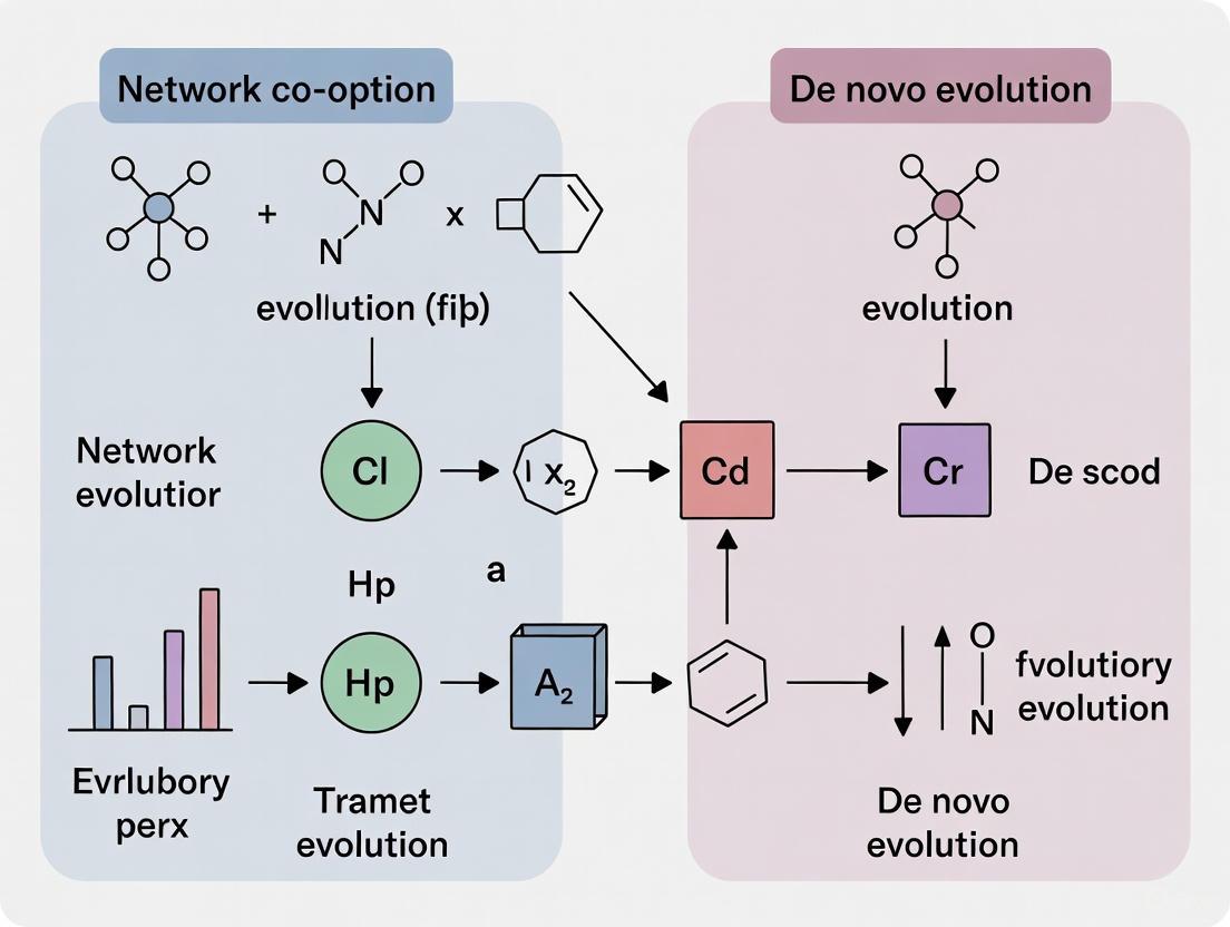
Visualizing the Conceptual Workflow
The following diagram illustrates the key decision points for classifying a genetic element as a product of co-option or de novo emergence.
Experimental Protocols & Methodologies
Protocol for Validating Co-option in a Toxin-Antitoxin System
This protocol is adapted from experimental work using the Evo genomic language model to generate and validate synthetic genetic systems [3].
Objective: To test the function of a predicted toxin-antitoxin (TA) pair generated through a co-option prompting strategy.
Materials:
- Generated toxin (e.g., EvoRelE1) and antitoxin sequences.
- Appropriate bacterial strain (e.g., E. coli).
- Growth media and incubator.
- Expression vectors with inducible promoters.
- Spectrophotometer for OD600 measurements.
Procedure:
- Cloning: Clone the generated toxin and antitoxin genes into separate expression vectors under the control of inducible promoters (e.g., pBAD or pTet).
- Transformation: Co-transform the toxin and antitoxin plasmids into the bacterial host strain.
- Growth Inhibition Assay:
- Inoculate cultures and grow to mid-log phase.
- Induce toxin expression while maintaining repression of the antitoxin.
- Monitor bacterial growth by measuring optical density at 600 nm (OD600) over 4-8 hours.
- Include control cultures where neither gene is induced, and where only the antitoxin is induced.
- Rescue Assay:
- Induce toxin expression and observe growth inhibition.
- After 2 hours, induce antitoxin expression.
- Monitor OD600 to assess recovery of bacterial growth.
- Data Analysis:
- Calculate relative survival by comparing the final OD600 of the experimental culture to the non-induced control.
- A functional toxin will show significant growth inhibition (e.g., ~70% reduction), and a functional antitoxin will rescue growth upon its induction [3].
Workflow for Semantic Design of Co-opted Circuits
The diagram below outlines the "semantic design" workflow for generating novel, functional genetic circuits by prompting a genomic language model with contextual information [3].
Troubleshooting Guide & FAQs
Design and In Silico Analysis
Q: My generated sequences from the language model show low novelty and are highly similar to known natural sequences. How can I increase diversity?
- A: Adjust the sampling parameters of the model (e.g., increase temperature) to encourage exploration. Employ stricter novelty filters in your post-processing pipeline, requiring lower percentage identity to known sequences in databases like NCBI [3] [1]. Use more diverse or less conserved genomic contexts in your initial prompts.
Q: In silico protein interaction prediction fails to show complex formation for my generated toxin-antitoxin pair. Should I discard these candidates?
- A: Not necessarily. Computational predictions can yield false negatives. If the sequences were generated from a functional context, proceed to low-throughput experimental validation. The interaction interface might be novel and not recognized by standard prediction tools [3].
Experimental Validation
Q: In the growth inhibition assay, I observe no toxicity when the putative toxin is expressed. What are potential causes?
- A:
- Lack of Function: The generated sequence may not encode a functional protein.
- Expression Issue: Verify protein expression via Western blot. Check that the induction system is working correctly.
- Codon Usage: The generated sequence may use codons that are rare in your expression host, impairing translation. Consider codon optimization.
- Target Specificity: The toxin may be specific to a bacterial strain different from your experimental model.
Q: The antitoxin fails to neutralize the toxin in the rescue assay. What could be wrong?
- A:
- Stoichiometry: The expression level of the antitoxin may be insufficient. Titrate the induction level for both toxin and antitoxin.
- Kinetics: The antitoxin might need to be expressed before or concurrently with the toxin to form a complex. Modify the timing of induction.
- Non-specific Interaction: The generated pair may not form a specific, stable complex despite being generated from the same context.
Data Interpretation and Classification
Q: I have a functional genetic element with no homologs in databases. Can I immediately classify it as de novo?
- A: No. The absence of evidence is not evidence of absence. Use comparative genomics across closely related species to confirm the absence of the sequence is not due to gaps in genome sequencing or annotation [1]. Additionally, investigate if the element could be a highly diverged product of an ancient duplication event, which can be misidentified as de novo [1].
Q: How do I demonstrate that a circuit was co-opted rather than evolved de novo?
- A: Provide evidence for the preexisting source. This can include:
- Identifying homologous circuit components in other species with different, ancestral functions.
- Showing that the core regulatory logic (e.g., promoter architecture, transcription factor binding sites) is conserved from a source circuit.
- Demonstrating that the new function relies on molecular interactions (e.g., protein-protein interactions) that existed in the ancestral system.
The Scientist's Toolkit: Essential Research Reagents
Table 2: Key Reagents for Studying Network Co-option
| Research Reagent / Tool | Function / Application | Examples / Notes |
|---|---|---|
| Genomic Language Models (e.g., Evo) | In-context generation of novel functional sequences by learning multi-gene relationships in prokaryotic genomes [3]. | Evo 1.5 model can perform "genomic autocomplete" and semantic design [3]. |
| Inducible Expression Systems | Controlled, separate induction of genetic circuit components (e.g., toxin and antitoxin) for functional testing [3]. | pBAD (arabinose-inducible), pTet (tetracycline-inducible). |
| Model Organisms | Versatile chassis for cloning and testing the function of synthetic genetic circuits. | Escherichia coli, Bacillus subtilis, Salmonella enterica [3]. |
| Sequence Databases | For homology searches and novelty assessment of generated sequences [1]. | NCBI GenBank, RefSeq [1]. |
| Genetic Design Automation (GDA) Tools | In silico design, modeling, and analysis of genetic circuits prior to physical construction [4]. | Cello 2.0 for automated circuit design [4]. |
| Plasmid Repositories | Source of standardized, well-characterized biological parts (promoters, RBS, etc.) for circuit construction. | Addgene repository [4]. |
The study of de novo gene evolution challenges the long-held belief that new genes arise exclusively from pre-existing genes through mechanisms like duplication. Instead, it reveals that genes can originate from scratch, emerging from ancestrally non-coding DNA sequences [5]. This process involves the transformation of non-functional genomic regions into sequences that encode functional proteins or RNAs, which then become integrated into the organism's genetic regulatory networks [6] [7].
For researchers in evolutionary biology and drug development, distinguishing true de novo origination from the co-option of existing network components is a complex task. This technical support center provides targeted guidance, experimental protocols, and data interpretation frameworks to address the specific challenges you may encounter in this emerging field.
Frequently Asked Questions & Troubleshooting
FAQ 1: What are the primary challenges in confirming de novo gene origination and how can I address them?
- Challenge 1: Differentiating from unannotated coding sequences.
- Solution: Employ a rigorous comparative genomics pipeline. Compare your candidate gene's genomic locus against closely related species and outgroups. A true de novo gene should have no homologous coding sequence in the ancestral genome, though the non-coding locus will be alignable [5]. Utilize multiple genomic databases to rule out annotation errors.
- Challenge 2: Detecting low or tissue-specific expression.
- Solution: Leverage single-cell RNA sequencing (scRNA-seq). Bulk RNA-seq can mask expression that is restricted to rare cell types. For example, in Drosophila testes, many de novo genes are primarily expressed in spermatocytes [5]. scRNA-seq can precisely identify these specific expression patterns and confirm the gene is not merely transcriptional noise.
- Challenge 3: Demonstrating protein-coding potential and function.
- Solution: Combine mass spectrometry with ribosome profiling (Ribo-seq). A mass spectrometry-first approach can detect peptides translated from previously unannotated open reading frames (ORFs). Corroborate these findings with Ribo-seq data to show that the ORF is actively bound by ribosomes, providing strong evidence of translation [5].
FAQ 2: How can I determine if a de novo gene has been integrated into existing gene regulatory networks?
- Issue: The gene is expressed, but its regulatory basis is unknown.
- Investigation Protocol:
- Identify Cis-Regulatory Elements: Analyze the chromatin accessibility (e.g., via ATAC-seq) around the de novo gene's locus. Look for open chromatin regions and conserved promoter motifs, which may be shared with adjacent, established genes [6].
- Pinpoint Key Transcription Factors (TFs): Apply computational methods to scRNA-seq data to infer which TFs are active in the same cell types where your de novo gene is expressed [7]. Research indicates that only a subset of TFs, such as achintya and vismay in Drosophila, may act as master regulators for many de novo genes [7].
- Perform Functional Validation: Genetically perturb the candidate TFs (e.g., via knockout or knockdown) and use RNA sequencing to observe if the expression of the de novo gene is significantly altered. A linear, dose-dependent response in the de novo gene's expression to TF copy number variation is strong evidence of direct regulation [6].
- Investigation Protocol:
FAQ 3: My experimental validation of a de novo gene's function is inconclusive. What are common pitfalls?
- Pitfall 1: Using an inappropriate phenotypic assay.
- Guidance: Many de novo genes may have subtle, context-specific, or redundant functions. If a standard viability or growth assay shows no effect, consider assays for stress response, competitive fitness, or specific physiological processes relevant to the gene's expression context (e.g., sperm competition for testis-expressed genes) [5].
- Pitfall 2: Overlooking non-coding RNA functions.
- Action: Do not assume the gene functions only at the protein level. Investigate potential roles as a long non-coding RNA (lncRNA) or microRNA. Techniques like RNA Immunoprecipitation (RIP) can help identify if the RNA molecule itself interacts with proteins or other RNAs [3].
- Pitfall 3: Inadequate consideration of genetic background.
- Action: De novo genes can be polymorphic within a population [5]. Ensure you are using a well-characterized strain for functional assays and be aware that the gene's effect might be dependent on the specific genetic background.
Experimental Protocols for Key Methodologies
Protocol 1: Identification and Validation Using Population Genomics
This protocol is adapted from foundational work in Drosophila to identify de novo genes that are polymorphic within a population [5].
- Sample Preparation: Sequence the genomes and transcriptomes (e.g., from relevant tissues like testes) of multiple strains or individuals from the species of interest.
- Candidate Identification: Map transcripts to the genome and identify transcribed regions that lack homology to annotated genes in the reference genome.
- Comparative Genomics: Align the genomic locus of each candidate to the genomes of closely related species. Filter for sequences where the ORF is present but was non-genic in the common ancestor.
- Expression Analysis: Analyze transcriptomic data to determine expression levels and tissue-specificity. Highly expressed, fixed genes are strong candidates for functional, selected de novo genes [5].
- Validation: Use RT-PCR and Sanger sequencing to confirm the expression and structure of the candidate gene.
Protocol 2: Confirming Protein Coding with Mass Spectrometry
This protocol outlines a method to find evidence of translation for putative de novo genes [5].
- Sample Preparation: Prepare a protein extract from tissues or cell types where the candidate gene is highly expressed.
- Mass Spectrometry: Perform tandem mass spectrometry (LC-MS/MS) on the digested protein sample.
- Database Search: Search the mass spectrometry data against a custom database that includes the predicted protein sequences from all candidate de novo ORFs, in addition to the standard annotated proteome.
- Validation: Corroborate peptide identifications with high-stringency filters. Cross-reference hits with ribosome profiling data from the same tissue, if available, to strengthen the evidence for active translation.
Research Reagent Solutions
The table below summarizes key reagents and tools for studying de novo genes.
| Reagent/Tool | Primary Function | Key Application in De Novo Research |
|---|---|---|
| Single-cell RNA-seq (scRNA-seq) | Profiling gene expression at single-cell resolution. | Identifying cell-type-specific expression of de novo genes, ruling out transcriptional noise [5]. |
| Custom Mass Spectrometry Database | Identifying peptides from unannotated ORFs. | Detecting protein products of de novo genes that are absent from standard protein databases [5]. |
| BioTapestry Software | Modeling and visualizing Gene Regulatory Networks (GRNs). | Mapping the integration of de novo genes into regulatory circuits and modeling their interactions [8]. |
| Genomic Language Models (e.g., Evo) | In silico generation of functional genomic sequences. | Designing novel functional elements and exploring sequence space beyond natural evolution for comparative studies [3]. |
| idopNetworks Framework | Reconstructing personalized, dynamic GRNs. | Modeling how gene-gene interactions, including those with de novo genes, vary among individuals and over time [9]. |
Data Presentation and Workflow Visualization
Table 1: Key Characteristics of Established vs. De Novo Genes
This table helps differentiate de novo genes from traditional genes during analysis.
| Feature | Established Gene | De Novo Gene |
|---|---|---|
| Genomic Origin | Modification of pre-existing gene [5] | Ancestrally non-coding DNA [5] |
| Sequence Homology | Detectable across lineages | Limited or none in related species [5] |
| Regulatory Integration | Complex, multi-factor regulation | Often reliant on a few master transcription factors [6] [7] |
| Expression Pattern | Broad or well-defined | Frequently tissue-/cell-type-specific (e.g., testes) [5] |
| Protein Structure | Typically ordered domains | Often disordered, but can become structured [5] |
Workflow Diagram for Distinguishing De Novo Evolution
The diagram below outlines a logical workflow for validating a de novo gene, from discovery to functional analysis.
Validation Workflow for De Novo Genes
Regulatory Network Integration Diagram
This diagram illustrates how a de novo gene can be co-regulated with its genomic neighbors, a key concept for distinguishing its integration into the network.
Cis-Regulatory Co-regulation Model
Frequently Asked Questions
Q1: What is the fundamental conceptual difference between network co-option and de novo network evolution? Network co-option involves the re-deployment of an existing, functional gene regulatory network (GRN) into a new developmental context, space, or time. In contrast, de novo evolution builds new network connections and regulatory relationships from scratch, often through novel genetic mutations [10].
Q2: What are the primary experimental signatures that distinguish a co-opted network? A co-opted network shows immediate, simultaneous recruitment of multiple, interconnected genes in a new context, often upon manipulation of a single upstream "selector" transcription factor. The ectopic expression of this factor recapitulates a significant portion of the original phenotype (e.g., ectopic eye formation from eyeless misexpression) [10]. De novo traits lack this rapid, coordinated redeployment.
Q3: How can phylogenetic analysis help differentiate these evolutionary pathways? For a co-opted trait, deep phylogenetic analysis will reveal that the core GRN components and their regulatory linkages predate the novel trait, having functioned in a different ancestral context. For a de novo trait, the emergence of new regulatory genes and their specific interactions coincides with the origin of the trait itself [10].
Q4: What constitutes conclusive evidence for de novo evolution of a network? Conclusive evidence requires demonstrating that the core regulatory relationships between genes in the network are novel and lack homology to any pre-existing developmental program. This is often supported by the emergence of new regulatory genes and their specific cis-regulatory elements that arose concurrently with the new trait [10].
Q5: Why is the initial loss of tissue specificity a key diagnostic after a co-option event? Following co-option, the cis-regulatory elements (CREs) of the recruited network are activated in both the ancestral and the novel contexts. This immediate expansion of function leads to a loss of specificity and increased pleiotropy, which can be detected via comparative gene expression analyses [10].
Experimental Protocols for Distinction
Protocol 1: Ectopic Misexpression to Test Co-option Potential
Objective: To determine if a candidate "initiator" gene can recruit a putative network to a new developmental location.
Materials:
- Standard laboratory model organism (e.g., Drosophila, zebrafish).
- Molecular cloning reagents for transgenesis.
- GAL4/UAS or equivalent misexpression system.
- Antibodies for immunohistochemistry against key network components.
- RNA probes for in situ hybridization.
Methodology:
- Transgene Construction: Clone the coding sequence of the candidate initiator transcription factor (e.g., Antennapedia, eyeless) under the control of a tissue-specific promoter that is active in a neutral or naive ectopic location.
- Organism Transformation: Generate stable transgenic lines or use transient methods to introduce the construct.
- Phenotypic Analysis: Score the resulting phenotypes for the presence of ectopic structures. A homeotic transformation (e.g., leg forming where an antenna should be) is a strong indicator of wholesale network co-option [10].
- Molecular Validation: Use immunohistochemistry and in situ hybridization to document the ectopic activation of downstream genes within the putative co-opted network. The simultaneous recruitment of multiple downstream effectors supports a co-option mechanism.
Protocol 2: Comparative Cis-Regulatory Analysis
Objective: To trace the evolutionary history of network components and their regulation to establish homology.
Materials:
- Genomic DNA from species possessing the novel trait and closely related species that lack it.
- Chromatin Immunoprecipitation (ChIP) grade antibodies for key transcription factors.
- Next-generation sequencing facilities.
Methodology:
- CRE Identification: Use chromatin accessibility assays (e.g., ATAC-seq) and ChIP-seq against histone modifications to identify active candidate CREs for key network genes in the tissues of interest.
- Cross-Species Comparison: Compare the sequences and regulatory states of these CREs across species with and without the trait. For a co-opted network, homologous CREs will be active in different tissues across species.
- Functional Testing: Clone candidate CREs from multiple species into reporter constructs (e.g., GFP) and test their activity in the original versus the novel tissue context via transgenesis. A conserved ability to drive expression in the ancestral context, even in species that have evolved a new trait, supports co-option from that ancestral context.
Protocol 3: Network Perturbation and Pleiotropy Mapping
Objective: To quantify the degree of functional independence between a novel trait and its putative ancestral network.
Materials:
- CRISPR/Cas9 or RNAi resources for targeted gene disruption/knockdown.
- Phenotypic imaging and quantification software.
Methodology:
- Node Perturbation: Systematically knock out or knock down key genes within the network in the model organism.
- Phenotypic Scoring: Quantitatively assess the effects on both the novel trait and the ancestral trait where the network originally functioned.
- Pleiotropy Index: Calculate the correlation between phenotypic effects. A high correlation indicates strong pleiotropic constraint, consistent with a recent co-option event where specificity has not yet been restored. A low correlation suggests the network has evolved independence, which can occur over time after the initial co-option [10].
Table 1: Diagnostic Characteristics of Network Evolution Pathways
| Characteristic | Network Co-option | De Novo Evolution |
|---|---|---|
| Genetic Basis | Change in expression of existing "selector" gene; re-use of existing CREs [10]. | De novo gene birth and/or evolution of novel CREs and transcription factors. |
| Pace of Trait Origin | Rapid (few genetic changes) [10]. | Gradual (accumulation of many mutations). |
| Initial Network Topology | Entire existing sub-circuit recruited wholesale or partially [10]. | New connections formed step-by-step. |
| Phylogenetic Signal | Network components and linkages predate the novel trait [10]. | Network emergence coincides with trait origin. |
| Pleiotropy | Initially high, due to shared CREs [10]. | Initially low, as the network is trait-specific. |
| Ectopic Expression Outcome | Can produce a recognizable, albeit imperfect, ectopic phenotype [10]. | No coherent ectopic phenotype expected. |
Table 2: Key Research Reagent Solutions
| Reagent / Tool | Primary Function | Application in Distinguishing Pathways |
|---|---|---|
| GAL4/UAS System | Targeted gene misexpression. | Testing sufficiency of a single factor to recruit a network ectopically [10]. |
| CRISPR/Cas9 | Precise gene knockout. | Disrupting network nodes to test necessity and map pleiotropic effects. |
| ChIP-seq Antibodies | Genome-wide mapping of protein-DNA interactions. | Identifying direct regulatory targets and comparing cis-regulatory landscapes. |
| Single-Cell RNA-seq | Profiling gene expression at cellular resolution. | Characterizing network deployment with high specificity in complex tissues. |
| Phylogenetic Footprinting Software | Comparing CREs across species. | Identifying ancient versus newly evolved regulatory sequences. |
Visualization Schematics
Graphviz Diagrams
Evolutionary Origins and Historical Context
Frequently Asked Questions (FAQs)
Q1: What is the fundamental difference between network co-option and de novo evolution in evolutionary biology?
A1: Network co-option involves the reuse of existing gene regulatory networks (GRNs) in new developmental contexts, while de novo evolution describes the emergence of entirely new genes from previously non-coding DNA sequences. Co-option works with existing genetic "building blocks," whereas de novo evolution creates entirely new genetic elements [11] [5]. Co-option is considered an important mechanism for rapid evolutionary change because it allows complex traits to appear relatively quickly by repurposing existing developmental programs [11] [10].
Q2: What experimental evidence can help distinguish between these two mechanisms when I discover a novel trait?
A2: Several experimental approaches can help distinguish these mechanisms:
- Comparative Genomics: Identify if genes involved in the novel trait have homologs in related species and examine their ancestral functions. Co-opted genes will show sequence similarity and evidence of previous functions [12].
- Expression Analysis: Determine if gene expression patterns associated with the novel trait appear in other developmental contexts in the same organism, which suggests co-option [10] [13].
- Functional Testing: Use techniques like RNAi or CRISPR to disrupt candidate genes and test their necessity in both the novel and potential ancestral contexts [14].
- Regulatory Element Mapping: Identify whether cis-regulatory elements controlling novel trait genes are shared with other traits or are newly evolved [13].
Q3: What are the common methodological challenges in distinguishing co-option from de novo origins?
A3: Key challenges include:
- Ancestral State Reconstruction: Difficulty in accurately inferring ancestral gene functions and expression patterns, especially when dealing with deep evolutionary timescales [12].
- Rapid Sequence Divergence: Newly evolved genes may be misclassified as de novo when they actually diverged rapidly from existing genes, obscuring homology [15].
- Transcriptional Noise: Distinguishing functional de novo genes from non-functional transcription of non-coding regions [5] [15].
- Incomplete Genomic Data: Missing data from key transitional species can obscure evolutionary pathways [12].
Troubleshooting Experimental Challenges
Problem: Inconclusive results when testing whether a gene network was co-opted or newly evolved.
Solution: Implement a multi-evidence approach:
- Combine Phylogenetic and Expression Data: Use phylostratigraphy (gene age dating) alongside detailed spatiotemporal expression mapping [15].
- Test Regulatory Elements: Examine whether cis-regulatory elements controlling your candidate genes show evidence of previous functions or are entirely novel [13].
- Assess Network Context: Determine if the gene operates as part of a larger network that appears in other contexts, which would support co-option [10] [16].
Problem: Difficulty determining whether a novel gene is functional or represents transcriptional noise.
Solution: Apply convergent validation:
- Proteomic Validation: Use mass spectrometry to detect protein products [5].
- Ribosome Profiling: Confirm translation through Ribo-seq [15].
- Population Genetics: Test for signatures of selection using dN/dS ratios and population frequency analyses [15].
- Functional Screens: Implement CRISPR/Cas9 knockout experiments to assess phenotypic effects [15].
Key Diagnostic Features Comparison
Table 1: Diagnostic criteria for distinguishing evolutionary mechanisms
| Diagnostic Feature | Network Co-option | De Novo Evolution |
|---|---|---|
| Gene Origin | Preexisting genes with ancestral functions | Novel genes from non-coding DNA |
| Regulatory Elements | Often uses existing cis-regulatory elements with modified function | Frequently involves newly evolved regulatory elements |
| Evolutionary Pace | Relatively rapid, leveraging existing complexity | Typically slower, requiring entirely new functional elements |
| Sequence Signatures | High sequence similarity to ancestral genes | Often shorter sequences, lacking conserved domains |
| Network Context | Genes operate in known regulatory networks | Integration into existing networks may be incomplete |
Table 2: Molecular characteristics comparison
| Molecular Characteristic | Co-opted Elements | De Novo Elements |
|---|---|---|
| Protein Length | Typical length for their gene family | Often shorter proteins (<100 amino acids) |
| Protein Structure | Conserved domains and structures present | Frequently lack recognizable domains, higher intrinsic disorder |
| Expression Pattern | Broader expression across multiple tissues | Highly restricted, tissue-specific expression |
| Evolutionary Conservation | Orthologs identifiable in related species | Lineage-specific, lacking clear orthologs |
| GC Content | Typical for conserved genes | Often reduced GC content |
Experimental Protocols
Protocol 1: Identifying Co-opted Gene Networks
Purpose: To determine whether a novel trait evolved through co-option of existing gene networks.
Methodology:
- Gene Expression Profiling: Perform RNA in situ hybridization or single-cell RNA-seq across multiple tissues and developmental stages [13] [5].
- Comparative Analysis: Compare expression patterns of candidate genes between the novel trait and other body structures.
- Regulatory Element Testing: Use CRISPR/Cas9 to modify candidate cis-regulatory elements and test effects on both the novel trait and potential ancestral expression domains [13].
- Network Mapping: Construct gene regulatory networks using chromatin immunoprecipitation (ChIP) or similar methods to identify shared transcription factors [10].
Interpretation: Evidence for co-option includes: 1) Shared expression patterns between novel and ancestral traits, 2) Regulatory elements that function in multiple contexts, and 3) Similar network architecture between traits.
Protocol 2: Validating De Novo Gene Origins
Purpose: To confirm that a candidate gene truly originated de novo from non-coding DNA.
Methodology:
- Phylostratigraphy: Perform systematic BLAST searches against increasingly distant relative species to confirm absence of homologs [15].
- Synteny Analysis: Examine genomic context across related species to confirm non-genic origin [15].
- Transcriptome Validation: Verify expression through RT-PCR, RNA-seq, and Ribo-seq to confirm translation [5] [15].
- Functional Tests: Implement gene knockout (CRISPR/Cas9) and overexpression to assess phenotypic effects [15].
Interpretation: Strong evidence for de novo origin includes: 1) Absence of homologs in sister species, 2) Non-genic ancestral sequence, 3) Translation evidence, and 4) Functional effects on phenotype.
Research Reagent Solutions
Table 3: Essential research reagents and their applications
| Reagent/Technique | Primary Function | Application Context |
|---|---|---|
| Single-cell RNA-seq | Gene expression profiling at cellular resolution | Identifying subtle expression patterns suggesting co-option [5] |
| CRISPR/Cas9 | Targeted genome editing | Testing gene function and regulatory element activity [15] |
| Mass Spectrometry | Protein detection and characterization | Validating translation of putative de novo genes [5] |
| Chromatin Immunoprecipitation (ChIP) | Mapping transcription factor binding sites | Defining gene regulatory networks [10] |
| Whole-mount in situ Hybridization | Spatial localization of gene expression | Comparing expression patterns across tissues [13] |
| Ribosome Profiling (Ribo-seq) | Monitoring translation | Confirming protein-coding potential [15] |
Conceptual Diagrams
Evolutionary Pathways to Novelty
Experimental Decision Framework
Frequently Asked Questions (FAQs)
Q1: What is the core difference between evolutionary tinkering and engineering in the context of gene evolution?
Evolution works as a tinkerer, not an engineer. Unlike an engineer who uses blueprints and purpose-selected materials, evolution lacks deliberate intent and works by reusing, combining, and modifying existing genetic parts. This process, termed bricolage, involves the opportunistic rearrangement of available elements, such as through gene duplication and domain shuffling, to create new functions. In contrast, rational engineering is based on foresight and precise planning [17].
Q2: What are the primary molecular mechanisms of evolutionary tinkering?
Molecular tinkering employs several key mechanisms to generate novelty, primarily by recombining existing protein "Lego blocks" [17]. The table below summarizes these core processes.
| Mechanism | Description | Key Outcome |
|---|---|---|
| Gene Duplication [17] | Creation of extra gene copies that can acquire new functions. A primary source of genetic raw material. | Generation of gene families and functional diversification. |
| Domain Shuffling [17] | Creation of mosaic proteins through exon shuffling, gene fusion, or fission. | Production of novel proteins with new combinations of functional domains. |
| Alternative Splicing [17] | Generation of multiple mRNA variants from a single gene. | Increases proteome diversity from a finite set of genes. |
| De Novo Gene Birth [6] [5] | Emergence of new protein-coding genes from ancestrally non-genic DNA sequences. | Origin of entirely new genes not derived from pre-existing coding sequences. |
Q3: How can I experimentally distinguish a de novo gene from a missed gene annotation?
This is a common challenge in evolutionary genetics. A robust experimental protocol involves a multi-step validation process to rule out annotation errors and confirm genuine de novo origin. The workflow below outlines the key steps and decision points.
Q4: My analysis suggests a gene network was co-opted. What evidence is needed to support this hypothesis?
Substantiating network co-option requires convergent evidence from multiple lines of inquiry. The table below details the types of data and expected findings for a robust conclusion.
| Evidence Type | Description | Expected Finding for Co-option |
|---|---|---|
| Phylogenetic [5] | Trace the evolutionary history of the network components (genes, regulatory elements). | Network components are ancient, but their coordinated expression in a new context is lineage-specific. |
| Expression [6] [18] | Map gene expression patterns of the network across different tissues, developmental stages, and species. | The same core set of genes is expressed in two distinct developmental or environmental contexts. |
| Regulatory [6] | Identify transcription factors and cis-regulatory elements controlling the network. | Shared regulatory logic (e.g., same transcription factors) controls the network in its old and new contexts. |
| Functional [18] | Test the functional requirement of key network genes in the new context (e.g., via knockouts). | Disruption of core network genes compromises the function of the novel trait. |
Q5: Why is the testes a common site for identifying young de novo genes, and can I find them in other tissues?
The testes of organisms like Drosophila are a hotspot for discovering young de novo genes due to strong sexual selection pressures and potentially less constrained regulatory environments, making it a fertile ground for evolutionary innovation [5]. However, de novo genes are not exclusive to the testes. They have been identified in other contexts, including genes linked to brain development in humans [5]. The choice of tissue should be guided by the biological question, with a focus on tissues under strong selective pressures or those known for rapid evolutionary divergence.
Troubleshooting Guides
Issue 1: Distinguishing TrueDe NovoGenes from Annotation Artifacts
Problem: A candidate gene appears to be lineage-specific, but you suspect it may be an artifact of poor genome annotation or undetected homology.
Solution: Follow the multi-step experimental protocol outlined in FAQ #3. Key troubleshooting steps include:
- Verify with Multiple Genomic Alignments: Use several high-quality reference genomes from closely and distantly related species. A true de novo gene will have no identifiable coding sequence homolog in the ancestral genomic region.
- Check for Non-Coding Transcripts: Use RNA-seq data from outgroup species to ensure the ancestral locus is not a transcribed but non-coding RNA.
- Assess Protein Evidence: Use mass spectrometry data to confirm the gene is translated. For example, one study used a "mass spectrometry-first, ORF-focused computational approach" to validate nearly 1,000 previously unannotated protein products in Drosophila [5].
Issue 2: Low Confidence in Resolving Plasmid Sequences for Synthetic Biology Constructs
Problem: When using long-read sequencing (e.g., Oxford Nanopore) to verify genetic constructs, the consensus sequence has low-confidence bases, complicating the validation of engineered sequences.
Solution: This is common in regions with specific sequence motifs. The table below lists common sources of error and how to address them.
| Problem Motif | Description | Solution / Interpretation |
|---|---|---|
| Homopolymer Regions [19] | Long stretches of a single nucleotide (e.g., AAAAAA). | ONT is prone to indels here. Low confidence calls in a homopolymer region are expected. Validate with Sanger sequencing if precise length is critical. |
| Dcm Methylation Sites [19] | CC[A/T]GG sequences in the sample. | Errors often occur at the middle base. Be cautious when interpreting variants at these specific sites. |
| Dam Methylation Sites [19] | GATC sequences. | Similar to Dcm sites, these can cause sequencing errors. |
| Low Coverage [19] | Insufficient number of reads covering a base. | Aim for an average coverage of >20x for a highly accurate consensus. Improve DNA sample quality and concentration to yield more reads. |
Issue 3: Differentiating Network Co-option from Parallel Evolution
Problem: You observe similar gene networks functioning in two lineages. It is unclear if this is due to co-option of an ancestral network or independent parallel evolution of similar networks.
Solution: The key is to dissect the evolutionary history of both the components and the regulatory linkages.
- Construct a Detailed Phylogeny: For co-option, the core network genes themselves will be anciently homologous across the lineages. In parallel evolution, the genes themselves may be different but converged on a similar function.
- Analyze cis-Regulatory Elements: This is the most definitive step. If the same non-coding regulatory elements control the network's expression in both lineages, it provides strong evidence for co-option. Parallel evolution would likely involve different regulatory sequences.
- Test Deep Homology: If possible, perform cross-species transgenic experiments. For example, if a regulatory element from one lineage can drive the expression of a reporter gene in the novel context of a second lineage, it supports co-option from a shared, ancestral regulatory capacity [18].
The Scientist's Toolkit: Essential Research Reagents & Materials
This table details key reagents and their applications for research in evolutionary genetics, specifically for studying de novo genes and network co-option.
| Item | Function / Application in Research |
|---|---|
| Custom Oligonucleotides [20] | Chemically synthesized DNA strands for PCR, sequencing, probe generation, and synthetic biology to build and validate genetic constructs. |
| Single-Cell RNA-Seq Kits | Profiling gene expression at single-cell resolution. Crucial for mapping the precise expression of young de novo genes to specific cell types (e.g., in Drosophila testes) [6] [5]. |
| Model Organism Strains (e.g., D. melanogaster) | Used for genetic manipulation (knock-outs, transgenics) to test the function of candidate de novo genes and manipulated gene networks [5]. |
| Plasmid Sequencing Services | Verification of synthetic DNA constructs. Whole-plasmid sequencing (e.g., via Oxford Nanopore) confirms the integrity of cloned sequences, including de novo gene inserts [19]. |
| Mass Spectrometry Equipment | Validating the translation of de novo genes by detecting their protein products. A key step in moving beyond transcriptional evidence [5]. |
| COBRA Toolbox [21] | A MATLAB toolbox for constraint-based reconstruction and analysis of metabolic networks. Can model how new genes integrate into and affect existing metabolic pathways. |
Detection and Analysis: Experimental and Computational Approaches
Comparative Genomics and Phylogenetic Analysis
FAQs: Common Questions in Phylogenetic Comparative Genomics
Q1: Why is it essential to control for phylogenetic relationships in comparative genomics studies? Closely related species share genes due to common descent, meaning their genomes cannot be treated as independent data points in statistical analyses. Applying phylogeny-based methods accounts for this non-independence. Failure to do so can lead to incorrect biological conclusions, as similarities might be misinterpreted as independent evolutionary events rather than shared ancestry [22].
Q2: What is the difference between a GenBank (GCA) and a RefSeq (GCF) genome assembly? A GenBank (GCA) assembly is an archival record of an assembled genome submitted to an INSDC member (like DDBJ, ENA, or GenBank). A RefSeq (GCF) assembly is an NCBI-derived copy of a GenBank assembly that is maintained and curated by NCBI. RefSeq assemblies always include annotation, and they may not be completely identical to their source GCA assemblies if NCBI has made improvements [23].
Q3: How can I programmatically access genomic data from NCBI without encountering rate limits? The NCBI Datasets API and command-line tools are rate-limited. Without an API key, the default limit is 5 requests per second (rps). Using an NCBI API key increases this limit to 10 rps and helps NCBI monitor and troubleshoot issues more effectively [23].
Q4: My sequencing library yield is low. What are the primary causes? Low library yield can stem from several issues in the preparation process [24]:
| Cause | Mechanism of Yield Loss | Corrective Action |
|---|---|---|
| Poor Input Quality | Enzyme inhibition from contaminants (e.g., salts, phenol) or degraded DNA/RNA. | Re-purify input sample; use fluorometric quantification (e.g., Qubit) instead of just absorbance. |
| Fragmentation Issues | Over- or under-fragmentation produces fragments outside the optimal size range for adapters. | Optimize fragmentation parameters (time, energy) and verify the fragment size distribution. |
| Suboptimal Ligation | Poor ligase performance or incorrect adapter-to-insert ratio reduces library molecules. | Titrate adapter ratios; ensure fresh ligase and optimal reaction conditions. |
| Overly Aggressive Cleanup | Desired fragments are accidentally excluded during purification or size selection. | Adjust bead-to-sample ratios and avoid over-drying beads. |
Q5: What is an "atypical" genome assembly on NCBI? Atypical genomes are those flagged by NCBI for one or more problems relating to assembly quality, unusual size, or other flaws. These can be identified on NCBI pages by a warning icon (a yellow triangle with an exclamation point). Users can typically filter these assemblies out of their search results [23].
Troubleshooting Guide: Sequencing Preparation for Comparative Genomics
Effective sequencing is the foundation of reliable comparative genomics. This guide addresses common failure points.
Problem: High Duplication Rates in Sequencing Data
Failure Signals: Abnormally high levels of PCR duplicates in the sequencing data, leading to reduced library complexity and biased genomic coverage [24].
Root Causes and Solutions:
| Root Cause | Explanation | Solution |
|---|---|---|
| Over-amplification | Too many PCR cycles during library amplification preferentially amplify a subset of fragments. | Reduce the number of PCR cycles; use the minimum cycles necessary for adequate yield. |
| Insufficient Input DNA | Low starting material reduces the initial complexity of the library, making duplicates more likely. | Increase input DNA within the recommended range for the library prep kit. |
| Amplification Bias | Polymerase inefficiency or inhibitors cause uneven amplification across the genome. | Use a high-fidelity polymerase optimized for GC-rich regions; ensure input DNA is clean. |
Problem: Adapter Contamination in Sequences
Failure Signals: A sharp peak around 70-90 base pairs in the electropherogram (BioAnalyzer/TapeStation trace), indicating the presence of adapter dimers [24].
Root Causes and Solutions:
| Root Cause | Explanation | Solution |
|---|---|---|
| Inefficient Ligation | Adapters ligate to each other instead of the DNA insert due to suboptimal conditions. | Titrate the adapter-to-insert molar ratio to find the optimum; use fresh, active ligase. |
| Ineffective Size Selection | Adapter dimers are not adequately removed before the amplification step. | Optimize bead-based cleanup ratios or use gel electrophoresis for precise size selection. |
| Carryover Contamination | Adapters from a previous reaction contaminate the current one. | Use clean lab practices, including changing gloves and using filtered pipette tips. |
Experimental Protocols for Key Analyses
Protocol 1: Phylogenetically Controlled Analysis of Gene Gain
Objective: To test if the gain of a de novo gene is associated with a specific phenotypic trait while controlling for shared evolutionary history [22].
Methodology:
- Data Collection: Identify species with and without the de novo gene of interest from genomic databases. Assemble corresponding phenotypic data.
- Phylogeny Reconstruction: Construct a robust phylogenetic tree for your species set using conserved, single-copy orthologs.
- Character Mapping: Map the presence/absence of the de novo gene and the phenotypic trait onto the tree.
- Statistical Testing: Employ phylogenetically independent contrasts (PIC) or a phylogenetic generalized least squares (PGLS) model to test for a correlation between the gene's presence and the trait, using the tree to account for non-independence.
Protocol 2: Identifying Regulators ofDe NovoGenes
Objective: To identify transcription factors that act as master regulators of newly evolved de novo genes [6].
Methodology:
- Single-Cell Sequencing: Apply single-cell RNA sequencing (e.g., to tissues like the testis in Drosophila where many de novo genes are expressed).
- Computational Inference: Use computational tools to infer transcription factor activity and co-expression networks from the single-cell data.
- Genetic Manipulation: Engineer model organisms (e.g., fruit flies) to have varying copy numbers of the candidate transcription factors.
- Expression Validation: Perform RNA sequencing on the engineered organisms to observe linear shifts in the expression of the de novo genes, confirming the role of the transcription factors.
Visualization of Concepts and Workflows
Phylogenetic Control in Comparative Analysis
De Novo Gene Regulatory Network
The Scientist's Toolkit: Research Reagent Solutions
| Reagent / Resource | Function in Research |
|---|---|
| RefSeq Genome Assemblies (GCF) | Provides NCBI-curated and annotated genomes, serving as a standardized reference for comparative analyses [23]. |
| Phylogenetic Analysis Software (e.g., for PIC, PGLS) | Implements statistical models that control for shared evolutionary history, allowing correct inference of evolutionary correlations [22]. |
| Single-Cell RNA-Seq Kits | Enables the profiling of gene expression at the resolution of individual cells, crucial for identifying rare cell types that express de novo genes [6]. |
| High-Fidelity PCR Enzyme Kits | Used for library amplification with minimal error, reducing biases and artifacts in next-generation sequencing (NGS) library preparation [24]. |
| Bead-Based Cleanup Kits | Purifies and size-selects DNA fragments during NGS library prep to remove contaminants like adapter dimers and select the desired insert size [24]. |
Enhancer Mapping and Cis-Regulatory Element Identification
Frequently Asked Questions (FAQs)
Q1: My luciferase or STARR-seq assay in human cell lines shows unexpectedly high activity from interferon-signaling genes. What is the cause and how can I resolve this?
This is a documented systematic error. Transfection of plasmid DNA into many common human cell lines (e.g., HeLa-S3, GM12878) can trigger an innate immune response, activating the cGAS-STING pathway and inducing type-I interferon (IFN-I) expression. This causes enhancers near interferon-stimulated genes (ISGs) to show dominant, false-positive signals [25].
- Solution: Treat cells during transfection with kinase inhibitors to suppress this pathway. Using a combination of the TBK1/IKKε inhibitor BX-795 and the PKR inhibitor C16 has been shown to prevent ISG induction and remove these false-positive enhancer signals without affecting true enhancer activity [25].
Q2: Where in the genome should I look to find the enhancers for my gene of interest, avoiding arbitrary distance limits?
The search space can be narrowed in a principled way using topologically associating domains (TADs). A gene and its enhancers are typically located within the same TAD, a fundamental unit of 3D genome organization. The boundaries of TADs are often conserved across cell types, even if the internal interactions are cell-type-specific [26].
- Solution: Use publicly available Hi-C data from various cell types to delineate the TAD boundaries surrounding your gene. This confines your enhancer search to a specific, functionally relevant genomic interval, which can then be screened for candidate cis-regulatory elements using epigenetic marks [26].
Q3: My reporter assays show conflicting results between plasmid-based systems and genomic context. What could be wrong?
A common issue involves the plasmid backbone itself. In widely used reporter systems (pGL3/4 and STARR-seq), the bacterial origin of replication (ORI) can act as a potent, conflicting core promoter, with most reporter transcripts initiating within the ORI rather than the intended minimal promoter [25].
- Solution: Redesign your plasmid to use the ORI as the core promoter, placing it immediately upstream of the reporter gene and candidate enhancer library. This avoids transcriptional interference from multiple promoters and has been shown to improve signal-to-noise ratios in both luciferase assays and STARR-seq screens [25].
Q4: How can I definitively prove that a candidate sequence is an enhancer for a specific gene, rather than just being in proximity?
Definitive proof requires demonstrating that perturbing the candidate sequence directly affects the expression of the target gene in its native genomic context. The traditional approach of testing for activity on a plasmid is not sufficient to confirm a functional gene-enhancer relationship in vivo [26].
- Solution: Use epigenome editing techniques like CRISPR interference (CRISPRi). By targeting a catalytically dead Cas9 (dCas9) fused to a repressive domain (e.g., KRAB) to the candidate enhancer, you can inactivate it. If this inactivation leads to downregulation of your candidate gene, it provides strong causal evidence for the enhancer-gene link [26].
Troubleshooting Guides
Problem: Low Signal or High Background in Enhancer Activity Assays
| Potential Cause | Diagnostic Steps | Solution |
|---|---|---|
| Conflicting Core Promoters | Map transcription start sites of reporter transcripts; a high percentage initiating in the plasmid ORI indicates this issue [25]. | Redesign constructs to use the ORI as the single, defined core promoter [25]. |
| Weak or Cell-Type-Inappropriate Enhancer | Check chromatin accessibility (ATAC-seq) and enhancer marks (H3K27ac, H3K4me1) in your cell type to confirm the element is expected to be active. | Use a positive control enhancer known to be active in your cell type. Consider screening in a different, more relevant cell model. |
| Inefficient Transfection | Measure transfection efficiency with a control plasmid (e.g., GFP reporter). | Optimize transfection protocol (e.g., electroporation parameters, reagent-to-DNA ratio) or use a different delivery method. |
Problem: Difficulty Linking Enhancers to Target Genes
| Potential Cause | Diagnostic Steps | Solution |
|---|---|---|
| Search Space Too Large | The candidate enhancer and putative target gene are located in different TADs. | Use Hi-C or other 3D chromatin data to define the TAD containing your enhancer and prioritize genes within it [26]. |
| Lack of Functional Validation | Relying solely on proximity or correlation from chromatin interaction data. | Employ CRISPRi to knock down the enhancer and measure the impact on expression of all candidate genes within the TAD [26]. |
| Sparse Chromatin Contact Data | Individual Hi-C datasets are too sparse to reliably detect long-range or trans-chromosomal contacts [27]. | Use a meta-analytically integrated Hi-C map (meta-Hi-C), which aggregates hundreds of individual experiments to create a high-density contact network with superior power to predict functional relationships [27]. |
Experimental Protocols for Key Methodologies
This protocol provides a systematic workflow to identify enhancers for a specific gene.
- Delineate the TAD: Use publicly available high-resolution Hi-C data (e.g., from the ENCODE project) for multiple cell types to identify the conserved TAD boundaries that encompass your gene of interest.
- Identify Candidate Enhancers within the TAD: Generate or consult a genome-wide map of putative enhancers for your cell type. This can be done by analyzing ChIP-seq data for histone marks (H3K4me1, H3K27ac) and/or transcription factors, combined with assays for open chromatin (ATAC-seq/DNase-seq). Overlap these putative enhancers with the defined TAD to generate a shortlist of candidate regulatory elements.
- Validate Enhancer-Gene Link by Functional Perturbation: For each candidate enhancer, design sgRNAs to target them with a CRISPRi system (e.g., dCas9-KRAB). Transfert the sgRNAs and dCas9 repressor into your relevant cell type and measure the expression of the target gene using qRT-PCR or RNA-seq. A significant downregulation confirms a functional enhancer-gene relationship.
Workflow for mapping enhancers to a target gene.
This protocol outlines modifications to the STARR-seq method for more reliable enhancer screening in human cells.
- Library Design: Clone your candidate DNA fragments into a plasmid vector where the ORI is used as the core promoter, placed directly upstream of the reporter gene. This removes the conflicting minimal promoter and improves the signal.
- Transfection with Inhibitor Treatment: Transfect the STARR-seq library into your target cells (e.g., HeLa-S3) using your preferred method. Include BX-795 (TBK1/IKKε inhibitor) and C16 (PKR inhibitor) in the culture medium during and after transfection to prevent the IFN-I response.
- Sequencing and Analysis: Proceed with the standard STARR-seq protocol for RNA extraction, library preparation, and sequencing. Analyze the data, noting that interferon-related false positives should be significantly diminished.
Research Reagent Solutions
Table: Essential Reagents for Enhancer Mapping and Validation
| Reagent / Tool | Function / Application | Key Consideration |
|---|---|---|
| TBK1/IKKε Inhibitor (BX-795) & PKR Inhibitor (C16) | Suppresses false-positive enhancer signals from innate immune response in plasmid-based assays in human cells [25]. | Critical for STARR-seq and luciferase assays in many common cell lines (e.g., HeLa-S3). |
| ORI-as-Promoter Plasmid Backbone | Provides a single, strong core promoter for reporter assays, eliminating confounding transcription from the plasmid backbone [25]. | Improves signal-to-noise compared to traditional dual-promoter vectors. |
| dCas9-KRAB CRISPRi System | Enables targeted epigenetic silencing of candidate enhancers in their native genomic context to validate gene targets [26]. | Essential for establishing causal enhancer-gene relationships. |
| Meta-Hi-C Chromatin Contact Maps | High-density, aggregated chromatin interaction networks for human, mouse, and fly. Powerful for identifying long-range and trans-chromosomal gene-enhancer connections [27]. | Outperforms individual Hi-C datasets in predicting functional relationships like coexpression. |
| H3K27ac & H3K4me1 Antibodies | For ChIP-seq to map active enhancers and promoters genome-wide. H3K27ac marks active enhancers; H3K4me1 marks poised and active enhancers [28] [26]. | The "peak-valley-peak" pattern in H3K27ac data can help pinpoint the precise nucleosome-depleted enhancer core [26]. |
Data Presentation Tables
Table: Distinguishing Features of Enhancer Evolutionary Origins
| Feature | Network Co-option | De Novo Evolution |
|---|---|---|
| Molecular Mechanism | Repurposing of a pre-existing enhancer from another developmental context [29]. | Emergence of a new enhancer from previously non-regulatory DNA [30]. |
| Genomic Origin | Preexisting regulatory sequences, sometimes via transposable elements [29]. | Non-functional, non-coding sequences (e.g., decaying duplicated genes) [30]. |
| Sequence Signature | Often shows sequence conservation with the ancestral enhancer, though binding sites may be gained/lost [29]. | Lineage-specific sequence conservation; may be absent in ancestor [30]. |
| Functional Role | Links a gene into a pre-established regulatory network [31]. | Creates a novel node in the regulatory network, potentially for a new trait [31] [30]. |
| Example | Posterior lobe enhancers in Drosophila genitalia co-opted from posterior spiracle network [29]. | "Recycled Regions" in teleost fish derived from non-coding remnants of duplicated genes [30]. |
Table: Comparison of Chromatin Interaction Mapping Technologies
| Technology | Description | Key Application in Enhancer Mapping | Consideration |
|---|---|---|---|
| Hi-C | Unbiased, genome-wide mapping of all chromatin contacts [27]. | Defining TAD boundaries; identifying overall 3D genome structure [26]. | Very sparse for long-range/trans contacts in individual datasets [27]. |
| ChIA-PET | Protein-centric interaction mapping (e.g., Pol2 ChIA-PET) [32]. | Identifying enhancer-promoter interactions mediated by a specific protein. | Broad domains and super enhancers show higher connectivity [32]. |
| Capture Hi-C | Targeted Hi-C focusing on specific genomic regions of interest [27]. | High-resolution mapping of interactions for a pre-defined set of loci (e.g., GWAS hits). | Requires prior knowledge to select target regions. |
| Meta-Hi-C | Computational aggregation of thousands of Hi-C experiments into a single high-density map [27]. | Powerful identification of functional long-range and trans-chromosomal contacts that predict coexpression. | A reference resource that complements, but does not replace, cell-type-specific data [27]. |
Single-Cell RNA Sequencing for Regulatory Network Inference
Frequently Asked Questions (FAQs)
Q1: Why is single-cell RNA sequencing particularly powerful for inferring gene regulatory networks (GRNs) compared to bulk RNA-seq?
Single-cell RNA sequencing (scRNA-seq) enables the measurement of gene expression in thousands of individual cells, providing high-resolution data on cellular heterogeneity. This cell-to-cell variability reveals statistical relationships that can be used to infer regulatory dependencies. While bulk RNA-seq averages expression across cell populations, thus masking underlying heterogeneity, scRNA-seq can identify rare cell populations and trace lineage relationships, making it ideal for reconstructing the GRNs that underlie functional heterogeneity and cell-type specification [33] [34]. Furthermore, scRNA-seq allows for the design of combinatorial perturbation experiments (e.g., Perturb-seq), where mixtures of genetic perturbations can be assayed in a single reaction, providing an efficient means of inferring GRNs [35].
Q2: What are the primary computational methods for inferring gene regulatory networks from scRNA-seq data?
Several computational methods have been developed specifically for GRN inference from single-cell data. Key approaches include:
- The Inferelator: A method based on regression with regularization that infers regulatory relationships between transcription factors (TFs) and target genes. It can incorporate multitask learning and has been successfully applied to scRNA-seq data from budding yeast [35].
- PIDC (Partial Information Decomposition and Context): An algorithm that uses multivariate information theory to explore statistical dependencies between triplets of genes. It identifies regulatory relationships by quantifying how much information two genes provide about a third, which often outperforms pairwise methods [34].
- Bayesian Formulations: Methods like Bayesian Nonnegative Matrix Factorization (bNMF) can be used to infer the depth of cellular heterogeneity and identify subgroup memberships, which is a key step in understanding regulatory complexity [36].
Q3: What are common sources of technical artifacts in scRNA-seq data that can confound network inference?
Technical artifacts that can significantly impact downstream GRN inference include:
- Ambient RNA: Transcripts released from damaged or apoptotic cells that are captured in droplets along with intact cells, contaminating the true gene expression profile [37].
- Doublets/Multiplets: Instances where more than one cell is captured in a single droplet or well, leading to hybrid expression profiles that can be mistaken for novel cell states or incorrect regulatory connections [37] [38].
- Low-Quality Cells: Cells with a high percentage of mitochondrial reads or a low number of detected genes, indicative of broken cells or insufficient mRNA capture [37] [38].
- Batch Effects: Technical variations introduced by differences in sample processing, library preparation, or sequencing runs, which can create spurious correlations and obscure true biological signals [37].
Troubleshooting Guides
Problem 1: High Ambient RNA Contamination
Symptoms:
- Detection of cell-type-specific marker genes in cell types where they are not expected.
- Generally high background noise in gene expression data.
Solutions:
- Computational Removal: Use specialized tools to estimate and subtract the background ambient RNA profile.
- SoupX: Effectively removes ambient RNA contamination and is less dependent on precise pre-annotation, though it requires some user input regarding marker genes [37].
- CellBender: A tool suited for cleaning up noisy datasets and providing an accurate estimation of background noise, often showing superior performance compared to other tools [37].
- Experimental Optimization: During sample preparation, minimize cell lysis and the generation of free-floating RNA. Use viability staining and dead cell removal protocols to reduce the contribution from dying cells [39] [40].
Problem 2: Excessive Doublet Rates
Symptoms:
- Cells co-expressing well-established marker genes for distinct cell types (e.g., a cell expressing both T-cell and B-cell markers).
- Outlier cells with unusually high UMI (Unique Molecular Identifier) counts or numbers of detected genes [37] [38].
Solutions:
- Experimental Adjustment: Avoid overloading cells during library preparation. Refer to platform-specific guidelines (e.g., for 10x Genomics, loading the recommended number of cells is critical to control the multiplet rate) [38].
- Computational Detection and Removal: Employ doublet-detection algorithms, preferably using a combination of tools for robust identification.
- DoubletFinder: Has been shown to outperform other methods in terms of accuracy and its positive impact on downstream analyses like clustering [37].
- Scrublet: A scalable method suitable for large datasets [37].
- It is recommended to use these tools in conjunction with manual inspection of cells co-expressing markers of distinct lineages [37].
Problem 3: Low-Quality Cells Obscuring Biological Signals
Symptoms:
- A large fraction of cells with a low number of total genes or UMIs.
- Cells with a high percentage of reads mapping to mitochondrial genes.
Solutions:
- Apply Quality Control Filters: Filter the cell barcode matrix to remove low-quality cells based on established thresholds. The table below summarizes key metrics and typical filtering criteria, though these should be adjusted based on sample type and biology [37] [38].
Table 1: Quality Control Metrics for Filtering Low-Quality Cells
| Metric | Typical Indicator of Low Quality | Common Filtering Thresholds (Guide Only) |
|---|---|---|
| Number of Genes per Cell | Insufficient mRNA capture; empty droplet | Filter cells with gene counts significantly below the distribution median [37]. |
| Total UMI Counts per Cell | Insufficient mRNA capture; empty droplet | Filter cells with UMI counts significantly below the distribution median [37]. |
| Mitochondrial Gene Percentage | Broken or dead cells; cellular stress | Often 5% - 15%, but varies by species and sample type. Highly metabolically active tissues may have higher baseline levels [37] [38]. |
| Stress-Related Gene Signature | Cellular stress from dissociation or handling | Filter cells expressing high levels of pre-defined dissociation or stress-related gene sets [37]. |
- Regress Out Unwanted Variation: During data scaling, regress out factors such as total UMIs per cell and mitochondrial gene percentage to mitigate the impact of these technical confounders on downstream analysis [37].
The Scientist's Toolkit: Essential Reagents and Computational Tools
Table 2: Key Research Reagent Solutions and Computational Tools for scRNA-seq GRN Inference
| Item | Function/Benefit | Example Products/Tools |
|---|---|---|
| Droplet-Based scRNA-seq Platform | High-throughput encapsulation of single cells into droplets for parallel library preparation. | 10x Genomics Chromium, ddSEQ from Bio-Rad, InDrop from 1CellBio [33]. |
| scRNA-seq Kit with UMIs | Facilitates whole-transcriptome analysis from single cells. UMIs enable accurate quantification by correcting for PCR amplification bias. | SMART-Seq kits (Takara Bio) [40], 10x Genomics Chromium Kits [38]. |
| Cell Suspension Buffer | Preserves cell integrity and prevents RNA degradation or interference with reverse transcription. | EDTA-, Mg2+- and Ca2+-free PBS; BD FACS Pre-Sort Buffer [40]. |
| Ambient RNA Removal Tool | Computationally estimates and subtracts background noise from the gene expression matrix. | SoupX, CellBender [37]. |
| Doublet Detection Tool | Identifies and removes multiplets from the dataset to prevent false biological interpretations. | DoubletFinder, Scrublet [37]. |
| GRN Inference Algorithm | Reconstructs regulatory networks from the processed single-cell gene expression matrix. | The Inferelator, PIDC [35] [34]. |
Visualizing the Experimental and Analytical Workflow
The following diagram outlines the core workflow for a scRNA-seq experiment aimed at inferring gene regulatory networks, highlighting key steps from sample preparation to computational analysis.
Diagram 1: scRNA-seq GRN inference workflow.
Applying scRNA-seq to Distinguish Network Co-option from De Novo Evolution
A primary challenge in evolutionary biology is determining whether a novel trait arises from the co-option of an existing gene regulatory network (GRN) or the de novo evolution of new regulatory circuitry. Single-cell RNA sequencing provides a powerful framework to address this question by enabling the detailed comparison of GRNs across species, cell types, and conditions.
Key Analytical Strategies:
- Comparative GRN Reconstruction: By applying GRN inference algorithms (like the Inferelator or PIDC) to scRNA-seq data from homologous tissues or cell types in different species, researchers can identify conserved network motifs. The presence of a conserved core network underlying a novel trait in a derived species strongly suggests co-option [35] [34].
- Mapping Cellular Phylogenies: Single-cell data allows for the inference of lineage trajectories (e.g., via pseudotime analysis). Mapping the activity of inferred GRNs onto these lineages can reveal if a new cell fate is associated with the rewiring of an ancestral developmental pathway (co-option) or the emergence of a unique regulatory program [33].
- Assessing Network Hierarchy: Bayesian model comparison frameworks, such as bNMF, can help determine the "depth of heterogeneity"—the number of distinct cell states or subtypes present in a sample. This can reveal whether a novel cell type is a subtle variant of an existing one (hinting at co-option) or a fundamentally distinct class, which could be consistent with either co-option or de novo evolution, requiring further investigation [36].
Visualizing the Core Evolutionary Question:
The following diagram contrasts the hypotheses of network co-option and de novo evolution, illustrating how scRNA-seq can help distinguish them.
Diagram 2: Co-option vs. de novo evolution.
Troubleshooting Guides
Guide 1: Addressing Poor Correlation Between Omics Layers
Problem: Expected strong correlations between differentially expressed transcripts and their corresponding proteins are not observed in your dataset.
Background: A lack of concordance between transcriptomic and proteomic data is a frequent challenge. This can arise from biological reasons (e.g., post-transcriptional regulation, differing turnover rates) or technical artifacts [41] [42].
Troubleshooting Steps:
- Repeat the Experiment: Unless cost or time-prohibitive, repeat the experiment to rule out simple human error or one-off technical failures [43].
- Verify Data Quality and Preprocessing:
- Equipment and Reagents: Check that mass spectrometers and other equipment are properly calibrated. Confirm reagents have been stored correctly and have not degraded [43].
- Normalization and Batch Effects: Apply appropriate normalization techniques (e.g., log-transformation, quantile normalization) to each omics dataset separately. Use batch effect correction tools like ComBat to remove technical variation unrelated to biology [41] [44].
- Check Your Biological Assumptions:
- Time Delays: Consider the temporal relationship between mRNA transcription and protein translation. A time-series experiment may be necessary to capture delayed correlations [42].
- Plausible Biology: The discordance may be biologically real. Re-examine the literature to see if strong transcript-protein correlation is expected for your system and genes of interest [43].
- Start Changing Variables (One at a Time):
Guide 2: Troubleshooting a Multi-Omics Workflow for Biomarker Discovery
Problem: An integrated multi-omics analysis fails to yield a robust, interpretable biomarker signature for distinguishing disease states.
Background: Biomarker discovery requires the fusion of proteomic and metabolomic features to enhance sensitivity and specificity compared to single-omics approaches [44].
Troubleshooting Steps:
- Confirm the Experiment Actually Failed:
- Evaluate if the negative result is scientifically plausible. A dim signal could indicate a problem with the protocol, or it could mean the molecular event is not detectable in your sample type [43].
- Ensure Appropriate Controls:
- Include positive controls (e.g., a sample with a known strong disease signature) to confirm your experimental and analytical workflow is capable of detecting a signal [43].
- Refine Data Integration and Modeling:
- Algorithm Selection: If using a machine learning model, try different algorithms (e.g., MOFA2 for factor analysis, mixOmics for multivariate statistics) that may be more suited to your data structure [41] [44].
- Feature Selection: Overly complex models can overfit. Implement stricter feature selection prior to integration to focus on the most meaningful variables [42].
- Validate with Targeted Methods:
- Use targeted proteomics (e.g., PRM) and metabolomics (e.g., NMR) on an independent sample cohort to confirm the validity of biomarkers identified in an untargeted discovery screen [44].
Frequently Asked Questions (FAQs)
Q1: What is the core conceptual difference between network co-option and de novo evolution in the context of multi-omics?
A: Network co-option involves the re-deployment of an existing, functional gene regulatory network (GRN) to a new developmental context (e.g., a different tissue or time). This is observed in multi-omics data as a shared set of interconnected transcripts, proteins, and metabolites across two distinct biological processes. For example, in Drosophila, the larval posterior spiracle GRN was co-opted to the male genitalia, and later to the testis mesoderm [10] [45]. In contrast, de novo evolution typically involves the emergence of new genetic elements or the gradual, independent wiring of new regulatory interactions. Multi-omics signatures would show a unique, context-specific network without strong parallels to other established networks in the organism.
Q2: How can I practically distinguish network co-option from other phenomena using multi-omics data?
A: You can distinguish them through specific analytical approaches on your integrated data [10] [45]:
- Identify Shared regulatory elements: If you have genomic data, check if the same cis-regulatory elements (CREs) control gene expression in both the ancestral and novel contexts. This is a strong indicator of co-option.
- Construct Comparative Networks: Build correlation or co-expression networks (e.g., using WGCNA or xMWAS) for both contexts. Co-option is suggested if you find highly similar network modules (clusters of interconnected genes/proteins/metabolites) in both networks [46] [42].
- Check for "Interlocking": Analyze if changes to the network in one context (e.g., a novel gene expression pattern) are mirrored in the other, even if it provides no selective advantage there. This "interlocking" is a hallmark of recent co-option [45].
Q3: My multi-omics data comes from different sample cohorts (non-matched). Can I still integrate it?
A: Yes, but your choice of integration method is critical. Non-matched samples preclude simultaneous integration methods that require a single data matrix. You must use step-wise (or sequential) integration approaches [41]. In this paradigm, you:
- Analyze each omics dataset independently to generate results (e.g., lists of differentially expressed genes and metabolites).
- Integrate these results in a subsequent step using methods like:
Q4: What are the most common pitfalls in multi-omics sample preparation, and how can I avoid them?
A: The primary challenge is reconciling the different biochemical requirements for extracting macromolecules [44]. Common pitfalls and solutions include:
- Pitfall: Using extraction protocols optimized for one molecule (e.g., RNA) that degrade others (e.g., metabolites).
- Solution: Whenever possible, use joint extraction protocols designed to simultaneously recover proteins, metabolites, and (if feasible) RNA/DNA from the same sample aliquot. This minimizes variability and ensures data comparability.
- Pitfall: Improper sample handling leading to degradation.
- Solution: Process samples rapidly on ice and use preservation techniques (e.g., flash-freezing in liquid nitrogen) that stabilize both unstable metabolites and labile proteins.
Q5: How do I choose between a correlation-based integration approach and a machine learning approach?
A: The choice depends on your study's goal [46] [41] [42].
- Use Correlation-Based Methods (e.g., Pearson/Spearman, WGCNA, xMWAS) when your goal is to understand relationships and build networks. These are excellent for hypothesis generation, identifying co-regulated modules, and constructing gene-metabolite interaction networks.
- Use Machine Learning/Artificial Intelligence (e.g., MOFA2, PLS-DA) when your goal is prediction, classification, or dimensionality reduction. These methods are powerful for building diagnostic models, identifying complex multi-omics biomarkers, and uncovering hidden factors that drive variation across all omics layers.
Experimental Protocols & Data Presentation
This table summarizes key results from a murine study that integrated transcriptomics and metabolomics 24 hours after total-body irradiation, demonstrating how quantitative data can be structured.
| Omics Layer | Dose | Dysregulated Entities | Key Dysregulated Genes / Metabolites | Enriched Pathways (GO/KEGG) |
|---|---|---|---|---|
| Transcriptomics | 1 Gy (Low) | 143 Genes (67 up, 76 down) | Pde5a | Not Specified |
| 7.5 Gy (High) | 2,837 Genes (1,595 up, 1,242 down) | Nos2, Hmgcs2, Oxct2a, 16 metabolic enzyme genes (e.g., Abat, Hmox1, Tymp) | Immunoglobulin production, cell adhesion, receptor activity | |
| Metabolomics & Lipidomics | 7.5 Gy (High) | Various amino acids, Phosphatidylcholines (PC), Phosphatidylethanolamines (PE), Carnitines | Dysregulated amino acids, PC, PE, carnitine species | Amino acid, carbohydrate, lipid, nucleotide, and fatty acid metabolism |
Table 2: Research Reagent Solutions for Multi-Omics Integration
This table details essential materials and tools used in multi-omics studies, with a focus on their function in integration and network analysis.
| Reagent / Tool Name | Function in Multi-Omics | Use Case in Network Co-Option Research |
|---|---|---|
| Liquid Chromatography-Tandem Mass Spectrometry (LC-MS/MS) | Primary technology for proteomics and metabolomics identification and quantification [44]. | Generate protein and metabolite abundance data to compare network states across different biological contexts. |
| Tandem Mass Tags (TMT) | Multiplexing technology allowing simultaneous quantification of proteins from multiple samples in a single MS run [44]. | Precisely compare protein levels from an ancestral organ and a putative co-opted organ, reducing batch effects. |
| Cytoscape | Open-source platform for visualizing complex molecular interaction networks [46]. | Visualize and compare gene-metabolite or gene-protein networks to identify shared modules indicative of co-option. |
| WGCNA (Weighted Gene Co-expression Network Analysis) | R package for identifying clusters (modules) of highly correlated genes; can be extended to metabolomics data [46] [42]. | Identify co-expressed gene modules that are preserved across two different tissues, suggesting shared regulatory programs. |
| xMWAS | Online tool that performs pairwise association analysis and builds integrated networks from multiple omics datasets [42]. | Construct and visualize a multi-omics network containing transcripts, proteins, and metabolites from co-opted networks. |
Multi-Omics Workflow and Co-Option Visualization
Multi-Omics Integration Workflow
This diagram illustrates a generalized workflow for integrating transcriptomic, proteomic, and metabolomic data, highlighting key steps from sample to biological insight.
Network Co-Option Conceptual Model
This diagram models the concept of gene network co-option, where an existing network is re-deployed in a new context, potentially leading to evolutionary novelty.
Troubleshooting CRISPR Screens
FAQ: Addressing Common CRISPR Screening Challenges
1. How much sequencing data is required for a CRISPR screen? It is generally recommended that each sample achieves a sequencing depth of at least 200x coverage. The required data volume can be estimated with the formula: Required Data Volume = Sequencing Depth × Library Coverage × Number of sgRNAs / Mapping Rate. For a typical human whole-genome knockout library, this translates to approximately 10 Gb of sequencing per sample [48].
2. Why do different sgRNAs targeting the same gene show variable performance? Gene editing efficiency is highly influenced by the intrinsic properties of each sgRNA sequence. Some sgRNAs may have little to no activity. To ensure reliable results, design at least 3–4 sgRNAs per gene to mitigate the impact of individual sgRNA performance variability [48].
3. What should I do if I see no significant gene enrichment in my screen? The absence of enrichment is often due to insufficient selection pressure during the screening process, not a statistical error. To address this, try increasing the selection pressure and/or extending the screening duration to allow for greater enrichment of positively selected cells [48].
4. How can I determine if my CRISPR screen was successful? The most reliable method is to include well-validated positive-control genes with corresponding sgRNAs in your library. If these controls are significantly enriched or depleted as expected, it indicates effective screening conditions. Success can also be evaluated by assessing cellular response (e.g., cell killing) and bioinformatics outputs like the distribution of sgRNA abundance [48].
5. Why are my knockout efficiencies low? Low knockout efficiency can stem from several common issues [49]:
- Suboptimal sgRNA design
- Low transfection efficiency
- High off-target effects
- Strong DNA repair activity in your cell line
6. What are the essential controls for a CRISPR experiment? Using proper controls is fundamental to interpreting your results [50]:
- Transfection Control: A fluorescent reporter (e.g., GFP mRNA) to confirm successful delivery of materials into cells.
- Positive Editing Control: A validated sgRNA with known high editing efficiency (e.g., targeting the human TRAC gene) to confirm your system is working.
- Negative Editing Control: Cells treated with a "scramble" sgRNA (with no genomic target), guide RNA only, or Cas nuclease only. This establishes a baseline for cellular phenotype without editing.
- Mock Control: Cells subjected to the transfection process without any CRISPR components to control for stress induced by the transfection method itself.
Troubleshooting Guide: Low Knockout Efficiency
| Problem | Potential Cause | Recommended Solution |
|---|---|---|
| Low Knockout Efficiency | Suboptimal sgRNA design [49] | Use bioinformatics tools (e.g., CRISPR Design Tool, Benchling) to predict optimal sgRNAs. Test 3-5 different sgRNAs per gene. [49] |
| Low transfection efficiency [49] | Optimize transfection method. Use lipid-based reagents (e.g., DharmaFECT, Lipofectamine 3000) or electroporation for hard-to-transfect cells. [49] | |
| High off-target effects [49] | Select sgRNAs with high specificity using design tools to minimize off-target binding. [49] | |
| Cell line-specific issues (e.g., high DNA repair activity) [49] | Use stably expressing Cas9 cell lines for more consistent and reliable editing. [49] | |
| Large Loss of sgRNAs | Insufficient initial library coverage [48] | Re-establish the CRISPR library cell pool with adequate coverage before beginning the screen. [48] |
| Excessive selection pressure during screening [48] | Reduce the selection pressure applied to the experimental group. [48] | |
| High Variation Between Replicates | Low correlation between replicates [48] | If reproducibility is low (Pearson correlation <0.8), perform pairwise comparisons and use Venn diagrams to find overlapping candidate genes. [48] |
Troubleshooting Reporter Assays
FAQ: Luciferase Reporter Assay Challenges
1. What is the principle behind a luciferase assay? Luciferase assays use enzymes that generate light (bioluminescence) by oxidizing a substrate. Firefly Luciferase (FLuc) requires its substrate luciferin, plus ATP and Mg²⁺, emitting light at 550-570 nm. Renilla Luciferase (RLuc) only requires oxygen to catalyze its substrate coelenterazine, emitting blue light (~480 nm). The dual-luciferase system uses a experimental reporter (often FLuc) and a control reporter (often RLuc) to normalize for variables like transfection efficiency [51].
2. Why is normalization critical in reporter assays? Transient transfection introduces variability from sources like differing cell numbers, transfection efficiency, and edge effects in multiwell plates. Normalization to a co-transfected internal control reporter (e.g., RLuc) accounts for this well-to-well variation, reducing coefficients of variation (CV) and making your data more reliable [52].
3. My luminescence signal is too high and saturating the detector. What should I do?
- Reduce the amount of transfected plasmid or the number of cells.
- Dilute the cell lysate before measurement.
- Decrease the integration time on your measurement instrument [51].
4. My luminescence signal is too low. How can I improve it?
- Increase the amount of transfected plasmid or the number of cells.
- Decrease the volume of the lysis buffer used.
- Ensure the reaction substrate is in excess and that all reaction components are balanced to room temperature for optimal enzyme activity [51].
- Check for low transfection efficiency or low promoter activity [53].
5. I see large variations between replicate wells. What could be the cause?
- Pipetting error: Ensure pipette tips are firmly sealed and avoid creating bubbles.
- Sample inhomogeneity: Centrifuge lysate samples before taking the supernatant for analysis [51].
- Edge effects: Be aware that heat and humidity can vary across a multiwell plate, affecting cell growth and transfection [52].
Key Reagents for Luciferase Assays
| Reagent | Function | Key Considerations |
|---|---|---|
| Reporter Plasmid (e.g., pGL4.20) | Carries the firefly luciferase gene under the control of your regulatory element of interest (promoter, enhancer, etc.). | For promoter studies, the vector lacks a promoter, allowing you to insert your sequence of interest. [51] |
| Control Reporter Plasmid (e.g., pRL-TK) | Provides a constitutively expressed internal control (e.g., Renilla luciferase) for normalization. | Use a weak promoter (like TK) to avoid interfering with the experimental reporter. A typical transfection ratio is 1:10 (control:reporter plasmid). [51] |
| Transfection Reagent (e.g., PEI, Lipofectamine 2000) | Delivers plasmid DNA into cultured cells. | Optimization is required for different cell lines. Low transfection efficiency is a major cause of poor signals. [53] [51] |
| Luciferase Assay Substrate (e.g., D-Luciferin) | The compound oxidized by firefly luciferase to produce light. | Protect from light and air. Prepare working solutions fresh and do not use beyond their stability window (e.g., 4 hours for Firefly Luciferase Glow Assay Solution). [53] |
| Cell Lysis Buffer | Breaks open cells to release the luciferase enzymes for measurement. | Use the buffer provided with the assay kit for optimal results. Non-optimized lysis buffers can cause low signal. [53] |
Workflow: Dual-Luciferase Reporter Assay
Experimental Protocols
Protocol 1: CRISPR Screen Validation
Objective: To functionally validate hits from a CRISPR screen in the context of network co-option studies.
Background: In network co-option, an existing gene regulatory network (GRN) is redeployed in a new context, which can initially reduce the tissue-specificity of the involved genes. Functional validation helps confirm if a co-opted gene is essential for the novel trait [10].
Materials:
- Validated sgRNAs targeting your candidate genes from the screen.
- Appropriate controls: non-targeting scramble sgRNA (negative control) and sgRNA targeting a known essential gene (positive control) [50].
- Cas9 protein or Cas9-expressing cell line.
- Transfection reagent or electroporator.
- Materials for assessing phenotype (e.g., cell viability assay, FACS, Western blot).
Procedure:
- Select Candidate Genes: Prioritize hits from your primary screen using statistical scores (e.g., RRA score from MAGeCK) and effect size (log-fold-change) [48].
- Re-test Individual sgRNAs: Transfert cells with individual sgRNAs (not the pooled library) targeting your candidate genes. Include positive and negative controls in the same experiment [50].
- Measure Phenotype: Apply the relevant selection pressure and quantify the phenotypic output (e.g., cell survival, reporter signal, differentiation marker).
- Validate Editing: Confirm gene knockout efficiency at the DNA level (e.g., by sequencing) and/or protein level (e.g., by Western blot).
- Interpret Results: A valid hit will show a phenotype consistent with the screen and have confirmed editing. The positive control should show the expected strong phenotype, while the negative control should resemble wild-type cells.
Protocol 2: Dual-Luciferase Reporter Assay
Objective: To study the interaction between a transcription factor and a target gene promoter, a key technique for probing GRN architecture and co-option events.
Materials:
- pGL4.20 vector (or similar firefly luciferase reporter vector).
- pRL-TK vector (or similar Renilla luciferase control vector).
- Plasmid expressing your transcription factor of interest.
- Cell culture of your chosen cell line.
- Transfection reagent.
- Dual-Luciferase Reporter Assay System kit.
- Luminometer.
Procedure:
- Clone Regulatory Element: Insert the promoter or enhancer sequence of your target gene into the multiple cloning site of the pGL4.20 vector [51].
- Plate Cells: Seed cells in a multi-well plate to reach 70-90% confluency at the time of transfection.
- Co-transfect Plasmids: For each well, transfert a mixture containing:
- Experimental group: Firefly reporter plasmid + transcription factor plasmid + control Renilla plasmid.
- Control group: Firefly reporter plasmid + empty vector plasmid + control Renilla plasmid. A typical mass ratio for firefly reporter plasmid to Renilla control plasmid is 10:1 [51].
- Incubate: Incubate cells for 24-36 hours to allow for gene expression [51].
- Prepare Lysates: Aspirate the culture medium, wash cells with PBS, and add passive lysis buffer. Gently shake the plate for 15 minutes, then transfer the lysate to a tube and centrifuge to remove debris [53].
- Measure Luminescence:
- Transfer lysate to an opaque 96-well plate.
- Inject the Firefly Luciferase substrate, wait, and measure the luminescence (FLuc signal).
- Then, inject the Stop & Renilla Luciferase substrate, wait, and measure the luminescence again (RLuc signal) [51].
- Analyze Data:
- For each well, calculate the normalized ratio: Firefly Luminescence / Renilla Luminescence.
- Compute the average normalized ratio for the control group.
- Divide the normalized ratio of each experimental well by the control group's average to get the relative activity, setting the control group to 1 [51].
Conceptual Framework: Network Co-option in Functional Validation
Understanding Network Co-option
In evolutionary and developmental biology, gene network co-option occurs when an existing gene regulatory network (GRN), which specifies one trait, is re-deployed in a new developmental context to produce a novel trait. This is initiated by a change in a regulatory factor that causes it to interact with pre-existing cis-regulatory elements of another network [10].
Immediate Outcomes of Co-option: When a network is co-opted, it can have several initial outcomes, which your functional validation experiments should seek to distinguish [10]:
- Wholesale Co-option: The entire network is redeployed, recapitulating the original trait in a new location (e.g., ectopic eye formation from eyeless gene misexpression).
- Partial Co-option: Only a subset of the network's genes are activated in the new context.
- Functionally Divergent Co-option: The co-opted network interacts with new factors in the novel cellular environment, producing a different phenotype.
Visualizing Co-option vs. de novo Evolution
This conceptual framework is critical for designing your functional validation experiments. If you are studying a novel trait, your CRISPR screens and reporter assays can help determine whether its genetic basis is a co-opted existing network or a newly evolved one.
Analytical Challenges and Resolution Strategies
Distinguishing True De Novo Origins from Rapid Divergence
Frequently Asked Questions
FAQ 1: What is the fundamental difference between a de novo gene and a rapidly diverged gene? A de novo gene originates from a previously non-coding genomic region, meaning its ancestral sequence was not functional [54] [55]. In contrast, a rapidly diverged gene originates from a pre-existing gene, often via duplication, but has accumulated mutations so quickly that its sequence similarity to its ancestor is no longer detectable [54] [55]. The key distinction lies in the ancestral state: non-coding for de novo versus coding for rapidly diverged.
FAQ 2: My candidate de novo gene has low, tissue-specific expression. Is this evidence for or against its functionality? Low and tissue-specific expression is a common characteristic of young, bona fide de novo genes and should not be automatically dismissed as noise [54] [15]. Key evidence to assess functionality includes:
- Purifying Selection: A significantly lower rate of non-synonymous mutations compared to synonymous substitutions (dN/dS < 1) [54].
- Translation Evidence: Support from ribosome profiling (Ribo-seq) data showing active translation [54] [56].
- Regulated Expression: Clear patterns of expression modulation during development or in response to stimuli, rather than constitutive low expression [54].
FAQ 3: How can I definitively rule out rapid divergence in my analysis? Synteny-based methods are considered the gold standard for this purpose [55]. This involves:
- Identifying the orthologous genomic region in closely related outgroup species.
- Demonstrating the absence of an intact open reading frame (ORF) in these ancestral regions.
- Identifying shared, disruptive mutations (e.g., stop codons, frameshifts) in the outgroup lineages that prevent the formation of the ORF [56]. The presence of such "common disablers" in the ancestor strongly supports a de novo origin over rapid divergence from a pre-existing coding sequence.
FAQ 4: What are the typical molecular features of a young de novo gene? Young de novo genes often exhibit a distinct profile compared to established genes [54] [15]:
| Feature | Typical Characteristic of Young De Novo Genes |
|---|---|
| ORF Length | Shorter |
| Exon Count | Fewer exons |
| Conserved Domains | Lacking recognizable domains |
| Protein Structure | Enriched in intrinsically disordered regions |
| Expression Level | Lower and more tissue-specific |
| Genomic Location | Often enriched in repetitive regions and sometimes on the X chromosome |
FAQ 5: A reviewer argues my de novo gene is a result of homology detection failure. How can I respond? This is a common and valid criticism. Strengthen your case by:
- Using Advanced Tools: Employ progressive whole-genome alignment tools (e.g., Cactus) that are more sensitive than traditional BLAST for detecting distant homology [15].
- Convergent Evidence: Integrate multiple lines of evidence beyond sequence similarity, such as the synteny analysis described above, and evidence of purifying selection [54] [55].
- Functional Validation: If possible, provide experimental data from reverse genetics (e.g., CRISPR knockdown) showing that the gene is essential or produces a specific phenotype, which strongly supports its functional reality [54] [56].
Experimental Protocols & Workflows
Protocol 1: A Robust Pipeline for Identifying De Novo Genes
This protocol synthesizes rigorous computational and experimental steps to distinguish true de novo origins [56] [55].
1. Candidate Compilation & Curation
- Compile candidate genes from public studies or your own transcriptomic data.
- Manually curate to confirm intact gene structures (promoters, splice sites) and ORFs.
2. Computational Validation of De Novo Origin
- Objective: To rule out rapid divergence and homology detection failure.
- Methods:
- Synteny Analysis: Reconstruct ancestral genomic sequences using whole-genome synteny alignments across multiple related species. The candidate's genomic region must be identifiable in outgroups [56] [55].
- Ancestral ORF Assessment: Demonstrate the absence of an intact ORF in the orthologous regions of ancestral sequences pre-dating the divergence of your focal lineage. Look for shared disruptive mutations ("common disablers") in outgroups [56].
- Homology Search: Perform a comprehensive search against the entire annotated proteome of your focal species and public databases (e.g., UniProtKB) to rule out a duplication-and-divergence origin [56].
3. Expression and Translation Validation
- Objective: To confirm the gene is transcribed and translated.
- Methods:
- RNA-Seq: Analyze data from multiple tissues or conditions to confirm expression. Use unique regions of the transcript to avoid false positives from pervasive antisense transcription [56].
- Ribo-Seq: Use ribosome profiling data to confirm active translation. Look for a distinct three-nucleotide periodicity in the ribosome-protected fragments, a key signature of translation [54] [56].
- Proteomics: Search mass spectrometry (MS) databases for peptides derived from the candidate ORF. Note: this may be biased against short proteins [54].
4. Functional Assessment
- Objective: To demonstrate biological significance.
- Methods:
Diagram 1: De novo gene validation workflow.
Protocol 2: Differentiating De Novo Birth from Network Co-option
This protocol addresses the specific context of distinguishing a novel gene from the co-option of an existing gene network.
1. Define the Novel Phenotype and Its Network
- Identify the gene regulatory network (GRN) associated with the novel trait in your focal species.
- Map the key nodes (transcription factors, effector genes) and their regulatory connections.
2. Interrogate the Ancestral State
- For Network Co-option: Trace the GRN components back to an ancestral network in a related species. Evidence for co-option includes:
- For De Novo Gene Involvement: Identify nodes within the GRN that are themselves de novo genes. Follow the identification protocol above to validate their origin from non-coding DNA.
3. Assess Specificity and Pleiotropy
- Co-option Initial Outcome: Network co-option often causes an immediate loss of tissue-specificity for the re-deployed cis-regulatory elements, increasing pleiotropy [10].
- De Novo Integration: A de novo gene integrating into a network may initially show high specificity. Its integration might be a consequence of the network's evolution after co-option or represent a entirely new module.
Diagram 2: Decision logic for de novo genes vs. network co-option.
Data Presentation: Quantitative Comparisons
Table 1: Comparative Features of Gene Origins
This table summarizes key quantitative and characteristic differences to aid in diagnosis [54] [56] [15].
| Feature | True De Novo Gene | Rapidly Diverged Gene | Gene via Network Co-option |
|---|---|---|---|
| Ancestral State | Non-coding DNA [54] [55] | Coding gene (via duplication, etc.) [54] | Pre-existing gene regulatory network (GRN) [10] |
| Sequence Homology | No detectable homology to any coding sequence [56] | Homology to ancestral gene may be detectable with sensitive methods [55] | Full homology of network nodes to their ancestral counterparts [10] |
| Syntenic Region | No intact ORF in ancestor; presence of "common disablers" [56] | Disrupted or highly divergent ORF in syntenic region | intact, functional GRN in an ancestral context [10] |
| Typical dN/dS Signal | Purifying selection in fixed genes [54] | Often a signal of positive selection post-duplication | Varies; nodes may be under stabilizing or new selective pressures |
| Genomic Context | Often associated with repetitive elements/TEs [54] [15] | Flanked by paralogs or pseudogenes | Defined by the architecture of the co-opted GRN |
| Primary Evidence | Synteny + absence of homology + expression/translation [56] [55] | Detection of eroded homology + phylogenetic shadowing | Recapitulation of ancestral phenotype in a new context via a regulatory change [10] |
Table 2: Key Molecular Properties of Young De Novo Genes vs. Canonical Genes
Data derived from studies in humans and plants show how de novo genes compare to established genes, supporting their identification [56] [15].
| Molecular Property | Young De Novo Genes | Canonical Genes | Notes |
|---|---|---|---|
| ORF GC Content | Comparable or slightly higher [56] | Standard | Higher GC content may facilitate exon origination [56]. |
| Protein Disorder | Higher (enriched in disordered regions) [56] [15] | Lower | Disorder allows flexible interactions and escapes strict folding constraints [15]. |
| C-terminal Hydrophobicity | Lower [56] | Higher | Lower hydrophobicity may promote protein stability by reducing proteasomal degradation [56]. |
| Translation Efficiency | Intermediate (lower than canonical) [56] | High | Appears to be optimized over evolutionary time [56]. |
| Essentiality (from knockdowns) | ~30% show essential/lethal phenotypes [54] [15] | Varies widely | A significant fraction become functionally important rapidly. In one human study, 57.1% suppression of tumor cell proliferation [56]. |
The Scientist's Toolkit: Research Reagent Solutions
| Reagent / Resource | Primary Function in De Novo Gene Research | Key Considerations |
|---|---|---|
| Ribo-seq (Ribosome Profiling) | Provides genome-wide evidence of active translation, confirming the protein-coding potential of a candidate ORF [54] [56]. | Look for characteristic 3-nucleotide periodicity in reads. Crucial for validating translation independently of protein abundance. |
| CRISPR-Cas9 (Knockout/Knockdown) | Functional validation through reverse genetics. Determines if the gene is essential or contributes to a specific phenotype [54] [56] [15]. | Phenotypes (e.g., lethality, morphological defects) provide the strongest evidence for biological function. |
| Cactus / Progressive Whole-Genome Aligners | Advanced synteny-based identification across divergent species, surpassing BLAST for detecting homology and establishing evolutionary trajectories [15]. | Essential for robustly distinguishing de novo genes from rapidly diverged ones. |
| Multi-species RNA-seq Datasets | Allows assessment of expression patterns and conservation in closely related species, helping to define the gene's age and lineage-specificity [56]. | Data from diverse tissues and developmental stages is critical. |
| AlphaFold2 / Protein Structure Predictors | Predicts 3D structure of novel proteins, revealing if they can achieve folded conformations despite lacking conserved domains [15]. | Useful for generating functional hypotheses about disordered regions and potential interaction interfaces. |
| dN/dS Calculation Software (e.g., PAML) | Quantifies the strength and type of natural selection acting on the gene, with dN/dS < 1 indicating purifying selection [54]. | Requires population genomic or multi-species sequence data. A key test for functional constraint. |
Overcoming Annotation Errors and Incomplete Genome Assemblies
FAQs: Addressing Common Experimental Challenges
FAQ 1: What are the most common types of errors in draft genome assemblies, and how can I detect them?
Draft genome assemblies often contain errors that can be categorized into two main types, which can be identified using specific tools:
- Small-scale errors: These include local single-nucleotide polymorphisms (SNPs) and small insertions-deletions (indels). They primarily affect genome accuracy and are often found in repetitive regions [57].
- Large-scale structural errors: These include misjoined contigs, where two unlinked genomic fragments are improperly connected. These errors can lead to the formation of erroneous scaffolds and have a major negative impact on downstream evolutionary or comparative genomic studies [57].
- Detection Tools: To identify these errors at single-nucleotide resolution, use reference-free tools like CRAQ (Clipping information for Revealing Assembly Quality). CRAQ maps raw sequencing reads back to the assembled sequence to pinpoint regional and structural errors by analyzing clipped alignments and coverage breaks [57]. For a targeted assessment of complex regions like immunoglobulin loci, the CloseRead pipeline can visualize local assembly quality and diagnose specific errors [58].
FAQ 2: My genome annotation is missing genes known to exist in my species. How can I improve its completeness?
A missing gene annotation often stems from an incomplete assembly or limitations in the annotation pipeline. To improve completeness:
- Assess Assembly Completeness: Use tools like BUSCO (Benchmarking Universal Single-Copy Orthologs) to evaluate the presence of highly conserved, single-copy orthologs. A low BUSCO score indicates a fragmented or incomplete assembly [59] [58].
- Incorporate Multiple Evidence Types: Leverage hybrid sequencing data. Use long-read sequencing (Oxford Nanopore or PacBio) to span repetitive regions and improve assembly continuity. Combine this with RNA-seq data to provide direct evidence of transcribed regions. Tools like StringTie can reconstruct transcripts from RNA-seq reads, which can then be incorporated into evidence-based annotation pipelines [59].
- Utilize Protein Evidence: Map known protein sequences from related species to your genome assembly using tools like miniprot to identify conserved coding regions that might have been missed by ab initio predictors [59].
FAQ 3: How can I distinguish between a true biological structural variant and an assembly error in a newly sequenced genome?
Distinguishing between real genetic variation and an artifact of the assembly process is critical.
- Cross-Platform Validation: The most robust method is to validate the putative variant using a different sequencing technology. For example, a structural variant called from Nanopore data can be verified with Illumina short reads or optical mapping data [60].
- Analyze Read Mapping Patterns: Use a tool like CRAQ. A true heterozygous site will show a mixture of alleles in the mapped reads. In contrast, a structural assembly error (misjoin) will typically be characterized by a complete loss of read coverage or a high concentration of clipped reads at the breakpoint [57].
- Independent Mapping: Techniques like Hi-C (chromatin interaction) data or optical maps provide independent, long-range scaffolding information. If the assembled structure is not supported by these physical maps, it is likely a misassembly [61].
FAQ 4: What is the most effective sequencing strategy for assembling a complex, repetitive genome de novo?
For complex genomes, a hybrid sequencing strategy is highly effective.
- The Strategy: Combine the high accuracy of Illumina short reads with the long-range connectivity of Oxford Nanopore Technologies (ONT) or PacBio long reads [60].
- The Workflow: Use the long reads to create a continuous assembly that spans repetitive regions. Then, use the high-accuracy short reads to "polish" this assembly, correcting small-scale errors inherent in long-read technologies. This approach balances completeness with base-level accuracy in a cost-effective manner [62] [60].
- Recommended Tools: Assemblers like NextDenovo are specifically designed for efficient error correction and assembly of noisy long reads, making them ideal for ONT data [63]. For the best results, benchmarking studies suggest using Flye for assembly followed by polishing with tools like Racon and Pilon [62].
FAQ 5: How does an incomplete genome assembly impact the study of gene regulatory network co-option?
An incomplete or erroneous assembly directly compromises the ability to accurately identify and study network co-option.
- Fragmented Networks: If key regulatory genes or their cis-regulatory elements are located in unassembled or misassembled regions, the gene regulatory network (GRN) will be incomplete. This makes it impossible to determine if a network was fully co-opted into a new developmental context [10].
- Misleading Evolutionary Inferences: An assembly error that falsely joins two unrelated genomic regions could create the illusion of a shared regulatory landscape, leading to a false conclusion of network co-option. Conversely, a fragmented assembly might break a truly co-opted network, making it appear as de novo evolution of a similar trait [10] [60].
- Loss of Specificity Analysis: A core outcome of network co-option is the initial loss of tissue-specificity for the co-opted genes, which may be restored over evolutionary time. An inaccurate assembly prevents the reliable identification of tissue-specific enhancers and promoters, hindering the analysis of this evolutionary dynamic [10].
Troubleshooting Guides
Guide 1: Diagnosing and Correcting a Misassembled Genomic Region
Problem: You suspect a structural error in your assembly after a gene model looks incomplete or a synteny plot shows a break compared to a reference.
Required Tools: CRAQ [57], IGV (Integrative Genomics Viewer), Hi-C data (optional but recommended).
Protocol:
- Identify Suspicious Regions: Run CRAQ on your draft assembly using the original long reads and/or short reads. The tool will generate a list of Clip-based Structural Error (CSE) sites, which are potential misjoin breakpoints [57].
- Visualize the Evidence: Load your assembly and the CRAQ output into a genome browser like IGV. Simultaneously load the BAM file of the raw reads mapped to the assembly.
- Inspect the Breakpoint: Navigate to the CSE coordinates. Look for the following definitive signatures of a misassembly:
- A sudden drop in read coverage to zero.
- A pile-up of clipped reads (where only part of a read aligns).
- A cluster of split-aligned reads [57].
- Validate with Hi-C (If Available): Check the Hi-C contact map for the region. A misjoin will often appear as an area with very few intra-scaffold contacts, indicating the two joined fragments are not actually physically linked in the genome [61].
- Correct the Assembly:
- Break the Contig: Use CRAQ's correction feature or a simple script to break the contig at the precise misjoin breakpoint identified in Step 3.
- Re-scaffold: Use the Hi-C data or optical maps to correctly orient and order the broken contigs within the scaffold [57].
Guide 2: Improving Gene Annotation in a Repetitive, Hard-to-Assemble Region
Problem: A specific gene family of interest (e.g., immune genes like immunoglobulins) is poorly annotated and fragmented in your assembly.
Required Tools: CloseRead [58], specialized assembler (e.g., NextDenovo [63]), MAKER/EvidenceModeler annotation pipeline [59].
Protocol:
- Targeted Assessment: Run the CloseRead pipeline, specifying the loci of interest (e.g., IGH, IGK, IGL for immunoglobulin). CloseRead will generate visualizations highlighting regions with poor read mapping, mismatches, and coverage breaks [58].
- Local Re-assembly: Extract all reads mapping to the problematic locus and its flanks. Perform a focused, local de novo assembly of this subset of reads using an assembler like NextDenovo, which is effective at handling repeats with noisy long reads [63] [58].
- Incorporate Supporting Evidence: For the local assembly, use all available data: long reads for continuity, short reads for polishing, and if possible, targeted RNA-seq data to capture full-length transcripts of the genes [59].
- Manual Curation and Integration: Replace the problematic region in the main assembly with the new, improved local assembly. Use the transcript evidence from RNA-seq to manually adjust and verify the gene models.
- Re-annotate: Run the improved assembly through an evidence-driven annotation pipeline like MAKER or EvidenceModeler, providing the RNA-seq evidence and protein homology data as input to generate a new, more accurate annotation [59].
Key Experimental Protocols and Workflows
Protocol 1: A Hybrid Genome Assembly and Validation Workflow
This protocol outlines a robust strategy for generating a high-quality genome assembly suitable for distinguishing network co-option.
Step-by-Step Methodology:
- DNA & RNA Extraction: Isolate high-molecular-weight DNA for long-read sequencing and total RNA for transcriptome sequencing.
- Multi-Platform Sequencing:
- De Novo Assembly: Assemble the long reads using a CTA (correction-then-assembly) tool like NextDenovo [63] or Flye [62].
- Assembly Polishing: Polish the initial assembly using the Illumina short reads. A recommended scheme is two rounds of Racon (long-read polisher) followed by one round of Pilon (short-read polisher) [62].
- Assembly Validation:
- Annotation: Run the validated assembly through the MAKER annotation pipeline, incorporating ab initio predictions, protein homology evidence, and the RNA-seq transcriptome assembled with StringTie [59].
The workflow below illustrates the hybrid assembly and validation pathway:
Protocol 2: A Framework for Analyzing Network Co-option
This protocol uses a high-quality assembly to investigate if a gene network was co-opted.
Step-by-Step Methodology:
- Define the Traits and Networks: Clearly define the two traits being compared (e.g., ancestral trait A and novel trait B) and identify the core gene regulatory network (GRN) for trait A using literature and functional genomics data [10].
- Map Expression in Novel Context: Using RNA-seq or in situ hybridization, test whether the core transcription factors and effector genes of GRN A are expressed in the novel location or developmental context of trait B. This is the initial evidence for co-option [10].
- Interrogate Cis-Regulatory Elements: Use ATAC-seq or ChIP-seq to map the chromatin accessibility and transcription factor binding sites for the genes in the network. In a co-option event, you expect the same cis-regulatory elements to be active in both traits, initially causing a loss of tissue-specificity [10].
- Test for Sufficiency: Use functional genetics (e.g., CRISPR) to misexpress the upstream "initiating" transcription factor of GRN A in the context of trait B. If this is sufficient to ectopically activate the rest of the network and induce traits of A in location B, it provides strong mechanistic support for co-option [10].
- Trace Evolutionary History: Perform comparative genomics with related species to determine when the network became active in the novel context, providing an evolutionary timeline for the co-option event.
The logical workflow for this analysis is shown below:
Research Reagent Solutions: Essential Tools for Genome Assembly and Annotation
The following table catalogs key bioinformatics tools and their functions for managing assembly and annotation challenges.
| Tool Name | Category | Primary Function | Relevance to Network Co-option Studies |
|---|---|---|---|
| NextDenovo [63] | Assembler | Efficient error correction and assembly of noisy long reads (e.g., ONT). | Provides the continuous, accurate assembly needed to reconstruct complete GRNs. |
| Flye [62] | Assembler | De novo assembler for long reads, often performs well in benchmarks. | Creates the foundational genome scaffold for downstream annotation. |
| CRAQ [57] | Quality Assessment | Identifies assembly errors at single-nucleotide resolution using clipped reads. | Ensures the genomic architecture (e.g., gene order, synteny) is correct, preventing false co-option inferences. |
| CloseRead [58] | Quality Assessment | Visualizes local assembly quality in complex regions (e.g., immunoglobulin loci). | Validates assembly of difficult but biologically critical gene families. |
| BUSCO [59] [58] | Quality Assessment | Assesses genome/completeness using universal single-copy orthologs. | A high score indicates a complete assembly, reducing risk of missing network genes. |
| MAKER [59] | Annotation Pipeline | Integrates ab initio gene predictions with evidence (EST, protein) for annotation. | The standard pipeline for generating comprehensive and accurate gene models. |
| EvidenceModeler [59] | Annotation Pipeline | Combines weighted evidence from multiple gene prediction sources. | Resolves discrepancies between different prediction algorithms to produce a consensus annotation. |
| StringTie [59] | Transcriptomics | Assembles RNA-seq reads into full-length transcripts. | Provides direct evidence of transcribed genes and splice variants for annotation. |
Comparative Data for Informed Decision-Making
Table 1: Benchmarking of Select Genome Assembly Tools
This table summarizes performance data from benchmarking studies to help select an appropriate assembler [63] [62].
| Assembler | Strategy | Best For | Key Strengths | Considerations |
|---|---|---|---|---|
| NextDenovo [63] | CTA (Correction then Assembly) | Noisy long reads (ONT); large, repeat-rich genomes. | High speed and high accuracy; effective at distinguishing gene copies in repeats. | Filters out very low-quality or chimeric reads. |
| Flye [62] | ATC (Assembly then Correction) | General long-read assembly; balanced performance. | Strong overall performance in benchmarks; good continuity. | Performance can be improved by pre-processing reads with Ratatosk [62]. |
| Canu [63] | CTA | Accurate assembly of challenging genomes. | Comprehensive read correction. | Can be computationally intensive and slower than newer tools [63]. |
| Necat [63] | CTA | Nanopore read assembly. | Fast correction and assembly. | Corrected read accuracy may be slightly lower than NextDenovo [63]. |
Table 2: Key Quality Metrics for Genome Assembly Assessment
A summary of critical metrics and their interpretation for evaluating your final assembly [59] [57] [58].
| Metric | Tool | What It Measures | Interpretation for a High-Quality Assembly |
|---|---|---|---|
| Contiguity | QUAST (N50) | The length for which contigs of that length or longer cover 50% of the assembly. | Higher N50 indicates a more continuous, less fragmented assembly. |
| Completeness | BUSCO | The percentage of conserved, single-copy orthologs that are fully represented in the assembly. | A score >95% is typically considered excellent for gene space. |
| Base Accuracy | Merqury [62] / CRAQ [57] | The number of small-scale (SNP/indel) errors in the assembled sequence. | A high QV score (e.g., >40) indicates low base error rate. |
| Structural Accuracy | CRAQ [57] / Hi-C | The number of large-scale misassemblies (misjoins, inversions). | A low number of CSEs (Clip-based Structural Errors) and a clean Hi-C map. |
| Repeat Resolution | LAI (LTR Assembly Index) [57] | The completeness of assembled repetitive elements, like LTR retrotransposons. | A higher LAI score indicates better assembly of repetitive regions. |
Addressing Pleiotropy and Specificity Loss in Co-opted Networks
Troubleshooting Guide: Common Experimental Challenges
This section addresses specific, high-priority issues researchers encounter when studying pleiotropy in co-opted networks.
FAQ 1: How can I distinguish true pleiotropy from a cascade of direct effects in a co-opted network?
The Problem: A gene is identified that affects multiple traits, but it is unclear if this is genuine pleiotropy (the gene directly influences each trait) or if the gene affects one primary trait that then indirectly affects others through the network.
The Solution: Use Causal Network Analysis with Mendelian Randomization principles to orient the direction of effects.
- Construct a Causal Network: Utilize algorithms like the Genome-Directed Acyclic Graph (G-DAG) to model the underlying causal relationships between your molecular phenotypes (e.g., metabolites, proteins) [64].
- Integrate Genetic Instruments: Incorporate loss-of-function (LoF) mutations or other genetic variants as instrumental variables to anchor the direction of causation within the network [64].
- Apply Structural Equation Modeling (SEM): Test the hypothesized pleiotropic effect. If the gene's effect on a downstream metabolite becomes non-significant when conditioning on an upstream, directly affected metabolite, this suggests an indirect effect (rejecting pleiotropy) rather than a direct, pleiotropic action [64].
Experimental Protocol:
- Step 1 - Genome-Metabolome Association: Perform a genome-wide association study (GWAS) or exome sequencing analysis on intermediate molecular phenotypes (e.g., metabolomics data). Adjust for covariates like age, gender, and population stratification [64].
- Step 2 - Causal Network Identification: Apply the G-DAG algorithm or similar to the adjusted molecular phenotypes to infer a causal network [64].
- Step 3 - Pleiotropy Assessment: For a gene of interest (e.g., one harboring a LoF mutation), use SEM to model its effect on multiple traits within the constructed network. Compare the model where the gene has direct paths to all traits against a model where its effects are mediated through a central node.
FAQ 2: My co-option experiment shows a novel expression pattern. How do I prove it arose from cis-regulatory co-option and not de novo evolution?
The Problem: A novel gene expression pattern is observed, but its origin is ambiguous. It could result from the co-option of an existing regulatory element or the de novo evolution of a new enhancer.
The Solution: A comparative and molecular dissection of the cis-regulatory region.
- Comparative Genomics: Identify the specific genomic region responsible for the novel expression pattern (e.g., via reporter gene assays in a model system). Then, compare this region across closely related species that both possess and lack the novel trait [13].
- Test for Preexistent Activity: If the novel enhancer activity is found to overlap with regions that have other, conserved enhancer activities, this provides strong evidence for co-option. The novel function was derived by exploiting the latent or cryptic activity of an extant regulatory sequence [13].
- Look for Transposition: Check if the enhancer has homology to transposable elements, which are a known source of pre-built regulatory information [13].
Experimental Protocol:
- Step 1 - Cis-regulatory Mapping: Use a series of reporter gene constructs (e.g., GFP) with nested deletions or mutations to pinpoint the minimal enhancer sequence sufficient to drive the novel expression pattern [13].
- Step 2 - Cross-Species Comparison: Introduce the orthologous enhancer sequences from sister species (both with and without the novel trait) into your model organism. An ancestral sequence with latent, low-level activity in the new pattern supports the co-option hypothesis.
- Step 3 - Site-Directed Mutagenesis: Identify transcription factor binding sites within the minimal enhancer. Mutate sites specific to the novel expression pattern to confirm their necessity while testing if the ancestral function is retained.
FAQ 3: How do I define and measure "pleiotropy" correctly in the context of network co-option for my publication?
The Problem: The term "pleiotropy" is used inconsistently across genetics, evolution, and molecular biology, leading to confusion in interpreting and describing results.
The Solution: Explicitly define the type of pleiotropy you are investigating [65].
- Molecular-Gene Pleiotropy: Focuses on the number of biochemical functions or molecular interactors a gene has. This can be measured by the number of protein-protein interactions or affected pathways in an omics study [65].
- Developmental Pleiotropy: Concerns the number of organismal traits or aspects of phenotype affected by a mutation. This is the mutational pleiotropy often observed in syndromic diseases and is central to questions about the genetic autonomy of traits [65].
- Selectional Pleiotropy: Relates to the number of separate components of fitness (e.g., fecundity, viability) a mutation affects. This is key for models like antagonistic pleiotropy in aging [65].
Recommendation: In network co-option research, the most relevant is often developmental pleiotropy. Clearly state that you are measuring the number of distinct phenotypic traits or network nodes affected by a genetic perturbation, and use causal network methods (see FAQ 1) to distinguish direct from indirect effects.
Table 1: Summary of Key Analytical Methods for Pleiotropy Assessment
| Method | Primary Function | Application in Co-option Research | Key Outcome / Metric |
|---|---|---|---|
| Causal Network (G-DAG) | Infers direction of causation between variables using genetic instruments [64]. | Mapping the causal flow of information in a co-opted network to identify primary targets. | A directed acyclic graph showing causal paths between molecular phenotypes. |
| Structural Equation Modeling (SEM) | Tests and estimates complex causal models with multiple dependent variables [64]. | Statistically assessing whether a gene's effect on multiple traits is direct (pleiotropy) or indirect. | Path coefficients & p-values; confirms/rejects pleiotropy hypothesis. |
| Cis-regulatory Dissection | Pinpoints and characterizes DNA sequences controlling gene expression [13]. | Determining the origin of a novel expression pattern (co-option vs. de novo). | Identifies minimal enhancer sequence and critical mutations. |
Table 2: Quantitative Data from Exemplary Pleiotropy Analysis [64]
This table summarizes findings from a study investigating Loss-of-Function (LoF) mutations and their effects on serum metabolomes, illustrating the process of pleiotropy assessment.
| Gene | Affected Metabolite(s) | Initial p-value | Causal Network Finding | SEM Conclusion (Pleiotropy?) |
|---|---|---|---|---|
| GPR97 | Oleate, Eicoseneate | Significant | Metabolites have a direct relationship [64]. | No. Effect on Eicoseneate was indirect via Oleate [64]. |
| BNIPL | Octanoylcarnitine, Decanoylcarnitine | Significant | Metabolites have a direct relationship [64]. | No. Effect on Octanoylcarnitine was indirect via Decanoylcarnitine [64]. |
| KIAA1755 | Eicosapentaenoate | 5E-14 | Gene is in the causal pathway to Triglycerides [64]. | Not directly tested; presented as a risk predictor in a causal chain. |
| CLDN17 | Multiple (Amino Acid & Lipid Pathways) | Significant | Not specified in detail. | Yes. Identified as having genuine pleiotropic actions [64]. |
Mandatory Visualizations
Causal Pathway for LoF Mutation
Enhancer Co-option Logic
The Scientist's Toolkit: Research Reagent Solutions
Table 3: Essential Materials for Pleiotropy and Co-option Research
| Research Reagent / Material | Function in Experimental Context |
|---|---|
| Loss-of-Function (LoF) Mutations | Used as instrumental variables in causal inference (Mendelian randomization) to establish the direction of effect from gene to intermediate phenotype [64]. |
| Intermediate Molecular Phenotypes (e.g., Metabolomics) | Integrated readouts of biological processes that functionally connect genetic variants to disease endpoints; ideal for GWAS and causal network construction [64]. |
| Reporter Gene Constructs (e.g., GFP/LacZ) | Used to visualize the activity of cis-regulatory elements in vivo, allowing for the mapping of enhancer sequences and their expression patterns across species [13]. |
| Closely Related Species (Phylogenetically) | Essential for comparative genomics to trace the evolutionary history of a novel expression pattern and distinguish co-option from other origins [13]. |
| Structural Equation Modeling (SEM) Software | Statistical tool used to test complex multi-trait hypotheses and assess whether a genetic variant's effect on multiple traits is direct (pleiotropic) or indirect [64]. |
Identifying Cryptic Regulatory Activities and Latent Functions
Troubleshooting Guide: Common Experimental Challenges
This section addresses specific technical problems researchers may encounter when designing experiments to distinguish network co-option from de novo evolution.
Q1: My transgenic reporter constructs show no expression in the novel tissue context. What could be wrong?
- Problem: Missing key transcription factors or repressive chromatin environment in novel context
- Solution:
- Verify transcription factor expression in target tissue via in situ hybridization or scRNA-seq [10]
- Test smaller regulatory subfragments that may escape repression [66]
- Treat with chromatin-modifying drugs (e.g., trichostatin A) to test epigenetic silencing
- Include positive control with known active enhancer from target tissue
Q2: How can I distinguish true co-option from parallel evolution of similar regulatory sequences?
- Problem: Convergent evolution versus genuine network reuse
- Solution:
- Perform cross-species transgenic assays with orthologous regulatory elements [66]
- Test for conserved transcription factor binding sites across taxa
- Use phylogenetic shadowing to identify deeply conserved non-coding elements
- Employ mutagenesis of putative binding sites to test functional conservation
Q3: My network analysis shows partial rather than wholesale co-option. How should I interpret this?
- Problem: Incomplete network redeployment complicating evolutionary interpretation
- Solution:
- Map network topology to identify core vs. peripheral components [10]
- Test whether partially co-opted nodes represent network "kernels" or interchangeable components
- Analyze gene expression patterns across developmental time series
- Consider that partial co-option may represent transitional evolutionary state
Q4: Cryptic regulatory activities are inconsistent across biological replicates. How to improve detection?
- Problem: Stochastic expression of latent functions
- Solution:
- Increase sample size to detect low-frequency expression events [66]
- Use more sensitive detection methods (single-cell RNA-seq, sensitive reporters)
- Test multiple environmental conditions that may induce cryptic functions [67]
- Employ computational methods to distinguish signal from noise in expression data
Frequently Asked Questions (FAQs)
Q: What exactly defines "cryptic" regulatory activity versus simply weak expression? A: Cryptic activities are phenotypically silent DNA sequences not normally expressed in wild-type populations but capable of expression through genetic or environmental changes. Unlike weak expression, cryptic functions are not part of the normal developmental program and may require specific conditions for revelation [66] [67].
Q: Can network co-option be distinguished from de novo evolution using genomic data alone? A: Genomic evidence can be suggestive but is rarely sufficient. Co-option typically shows:
- Preexistence of network components in ancestral context
- Conservation of regulatory linkages across species
- Experimental evidence of function in ancestral tissue Definitive distinction requires functional validation through comparative transgenic assays and perturbation experiments [66] [10].
Q: What are the most reliable experimental systems for studying cryptic regulatory evolution? A: Established model systems with:
- Well-characterized gene regulatory networks (e.g., Drosophila pigmentation) [66]
- Multiple closely-related species with phenotypic diversity
- Robust transgenic tools (e.g., Gorteria diffusa petal spots) [14]
- Available genomic resources and functional genomics tools
Q: How does the initial outcome of network co-option affect subsequent evolutionary potential? A: Initial outcomes fall along a spectrum with different evolutionary implications:
- Wholesale co-option: Rapid novelty but high pleiotropic constraints
- Partial co-option: Modular reuse with maintained specificity
- Functionally divergent: Immediate functional differentiation
- Aphenotypic: No immediate phenotype, evolutionary "raw material" [10]
Table 1: Quantitative Framework for Identifying Cryptic Regulatory Activities
| Experimental Approach | Key Measurable Parameters | Expected Results for Co-option | Expected Results for De Novo Evolution |
|---|---|---|---|
| Cross-species transgenic reporter assays | Expression pattern conservation | Cryptic patterns matching other species' explicit patterns [66] | No conserved regulatory capacity |
| Transcription factor binding site analysis | Binding site conservation & functionality | Pre-existing functional sites in ancestral context | Novel binding sites not present ancestrally |
| Network topology analysis | Connectivity patterns, centrality measures | Conserved network architecture across contexts [10] | Novel network connections |
| Expression threshold testing | Response curves to regulatory inputs | Similar dose-response relationships | Divergent regulatory logic |
| Epigenetic landscape mapping | Chromatin accessibility, histone marks | Pre-permissive chromatin in ancestral context [66] | Novel epigenetic states |
Table 2: Research Reagent Solutions for Key Experiments
| Reagent/Tool | Experimental Function | Example Application | Key Considerations |
|---|---|---|---|
| piggyBac-attB vector system [66] | Transgenic integration | Testing enhancer activities across species | Consistent genomic insertion context |
| Nuclear EGFP reporters | Quantitative expression imaging | Mapping spatial expression patterns | Nuclear localization for cell resolution |
| BioTapestry software [8] | GRN visualization & modeling | Comparing network architectures across traits | Standardized representation for cross-study comparison |
| scRNA-seq platforms | Single-cell transcriptomics | Identifying rare cell populations with cryptic expression | Sensitivity thresholds for low-abundance transcripts |
| CRISPR/Cas9 mutagenesis | Precise regulatory element editing | Testing necessity of specific binding sites | Off-target effects on regulatory landscape |
Detailed Experimental Protocols
Protocol 1: Identifying Cryptic Enhancer Activities Using Transgenic Reporters
Based on: Kalay et al. 2019 methodology for Drosophila yellow gene enhancer analysis [66]
Materials:
- Putative regulatory regions from multiple species (≥1kb fragments)
- piggyBac-attB vector with nuclear EGFP reporter
- attP-40 Drosophila line for consistent genomic insertion
- AscI and FseI restriction enzymes for cloning
Methodology:
- Amplify regulatory fragments using Phusion-Taq polymerase mix to prevent mutations
- Clone into sequencing vector (pGEM-T) and sequence verify all constructs
- Subclone into piggyBac-attB vector using AscI sites
- Insert nEGFP coding sequence downstream using FseI site
- Inject constructs into attP-40 Drosophila line
- Analyze at least 3 independent transgenic lines per construct
- Score expression patterns in pupal and adult stages
- Compare fragments across species for cryptic vs. explicit activities
Critical Parameters:
- Include overlapping fragments to detect distributed enhancer functions
- Test both 5' intergenic and intronic regions regardless of known enhancer locations
- Use identical genomic landing site for all constructs
- Blind scoring of expression patterns to prevent bias
Protocol 2: Distinguishing Network Co-option Through Comparative GRN Analysis
Based on: Gorteria diffusa petal spot evolution methodology [14]
Materials:
- Tissue from ancestral and novel contexts across multiple species
- RNA-seq library preparation kits
- In situ hybridization reagents
- CRISPR/Cas9 mutagenesis tools
Methodology:
- Perform comparative transcriptomics of ancestral and novel traits
- Identify co-expressed gene modules using WGCNA or similar approaches
- Map spatial expression patterns via in situ hybridization
- Test regulatory relationships through perturbation experiments
- Construct gene regulatory networks for each context
- Compare network topology using graph alignment algorithms
- Identify conserved "kernel" vs. context-specific "plug-in" components
- Validate necessity through targeted mutagenesis of regulatory elements
Validation Criteria:
- Orthologous genes show conserved expression in ancestral context
- Network connections are functionally conserved
- Minimal novel regulatory innovations required
- Phylogenetic distribution supports pre-existence
Visualizations
Cryptic Regulatory Activity Detection Workflow
Network Co-option vs De Novo Evolution Decision Framework
Types of Network Co-option Outcomes
Optimizing Parameters for Network Hierarchy Reconstruction
This technical support center provides troubleshooting guides and FAQs for researchers working on reconstructing gene regulatory network hierarchies, specifically in the context of distinguishing network co-option from de novo evolution.
Frequently Asked Questions & Troubleshooting Guides
Q1: Why does my reconstructed network fail to identify known master regulators of evolutionary young genes?
A: This often stems from inappropriate hyperparameters in your Graph Neural Network (GNN) or analysis pipeline.
- Problem: Key transcription factors, like achintya and vismay, which are instrumental for regulating de novo genes, are not identified in your results [7].
- Solution: Optimize the hyperparameters of your model. Use Bayesian Optimization to tune critical parameters, as it efficiently balances exploration and exploitation, building a probabilistic model to guide the search for optimal settings [68] [69]. Ensure your single-cell RNA sequencing data is of high quality, as the identification of these regulators relies on such data [7].
Q2: How can I enforce physical or biological constraints during network reconstruction to improve accuracy?
A: Consider using a framework that decouples constraint application from parameter regularization.
- Problem: Applying biological constraints (e.g., known conservation laws) directly via loss functions can conflict with other optimization goals and degrade performance [70].
- Solution: Implement a knowledge distillation approach, like the Physics structure-informed neural network (Ψ-NN). This method uses a teacher-student framework. The teacher network is trained with physical/biological constraints, and this knowledge is then distilled into a student network, which separately undergoes parameter regularization. This staged optimization avoids conflict and helps embed meaningful structures [70].
Q3: What is the most efficient way to search for an optimal network architecture when studying novel gene networks?
A: For complex searches, self-evolving frameworks that combine multiple strategies are often effective.
- Problem: Exhaustive search methods like Grid Search are too computationally expensive for exploring vast architecture spaces [71] [72].
- Solution: Utilize a framework like SEArch, which integrates network pruning, knowledge distillation, and neural architecture search (NAS). It iteratively modifies a simple network's structure with guidance from a teacher network, efficiently evolving towards an architecture that meets performance and size budgets [73].
Q4: How can I automatically extract and interpret a meaningful structure from a trained network model?
A: Apply clustering and structure extraction algorithms to the trained model's parameters.
- Problem: The internal structure of a trained neural network is often seen as a "black box" [70].
- Solution: After training, use clustering techniques on the model's parameter matrices. Converged parameter values can be grouped into distinct clusters. These cluster centers can then be used to reconstruct a new, more interpretable network architecture that retains physical or biological significance, as demonstrated in the Ψ-NN method for solving PDEs [70].
Q5: My model is overfitting to the gene expression data of a specific cell type. How can I improve its generalizability?
A: Adjust regularization hyperparameters and use validation techniques.
- Problem: The model performs well on training data but fails to generalize to data from other cell types or conditions.
- Solution: Tune regularization hyperparameters like Dropout Rate and L2 Regularization Strength. Increase their values to reduce overfitting [71]. Furthermore, employ robust cross-validation during training to ensure your model's performance generalizes to unseen datasets [72].
Experimental Protocols & Data Presentation
Table 1: Hyperparameter Tuning Methods Comparison
This table summarizes the core methods for optimizing your model's hyperparameters, a critical step in network reconstruction.
| Method | Key Principle | Best Use Cases | Computational Cost |
|---|---|---|---|
| Grid Search [74] [71] [72] | Exhaustively tests all combinations in a predefined set. | Small, well-defined hyperparameter spaces. | Very high, grows exponentially with parameters. |
| Random Search [74] [71] [72] | Randomly samples combinations from defined distributions. | Larger search spaces where some hyperparameters have low impact. | Lower than Grid Search; efficient with many parameters. |
| Bayesian Optimization [71] [68] [69] | Builds a probabilistic model to guide the search towards promising regions. | Expensive model training (e.g., deep learning); limited computational budget. | Moderate; reduces the number of training runs needed. |
| Genetic Algorithms [69] | Uses evolutionary principles (mutation, crossover) to evolve hyperparameter sets. | Complex, non-differentiable search spaces and multi-objective optimization. | Can be high due to population-based evaluation. |
Table 2: Key Hyperparameters for Deep Learning in Network Reconstruction
These hyperparameters govern the training process and significantly impact model performance in reconstructing networks.
| Hyperparameter | Function | Impact on Model | Common Values / Strategies |
|---|---|---|---|
| Learning Rate [71] [72] | Controls the step size during weight updates. | Too high: model may diverge. Too low: slow training. | Log-uniform distribution (e.g., 1e-5 to 1e-2); use decay schedules [71] [72]. |
| Batch Size [71] [72] | Number of samples processed before a model update. | Larger batches: faster, stable, but may generalize poorly. Smaller batches: noisy, can help escape local minima. | Powers of two (e.g., 32, 64); often tuned with learning rate [71]. |
| Dropout Rate [71] | Randomly disables neurons during training to prevent overfitting. | Too high: loses information. Too low: may overfit. | Typically between 0.2 and 0.5 [71]. |
| Number of Epochs [71] [72] | Number of complete passes through the training dataset. | Too few: underfitting. Too many: overfitting. | Use early stopping to halt training when validation performance stops improving [71]. |
| GNN-Specific: Hidden State Size [71] [68] | Size of the internal memory in graph network units. | Larger sizes capture more context but risk overfitting. | Often searched within ranges like [16, 32, 64, 128]. |
Protocol 1: Automated Hyperparameter Tuning using Bayesian Optimization
This methodology is crucial for optimizing Graph Neural Networks and other models used in cheminformatics and molecular property prediction [68].
- Define the Search Space: Specify the hyperparameters and their value ranges using statistical distributions (e.g., log-uniform for learning rate, uniform for dropout rate) [71].
- Select an Objective Function: Choose a metric to maximize (e.g., prediction accuracy) or minimize (e.g., validation loss). This function will evaluate each model configuration.
- Initialize the Surrogate Model: Begin by evaluating a few random hyperparameter combinations. Bayesian Optimization uses these to build a probabilistic model (surrogate), like a Gaussian Process, of the objective function [71] [69].
- Iterate and Select:
- Use the surrogate model to predict the most promising hyperparameter combination to evaluate next (balancing exploration and exploitation).
- Train and evaluate the model with this new combination.
- Update the surrogate model with the new result.
- Terminate and Select Best: Repeat Step 4 for a fixed number of iterations or until performance plateaus. Finally, select the hyperparameter set that achieved the best performance on the objective function.
Protocol 2: Network Structure Discovery via Knowledge Distillation (Ψ-NN)
This protocol is for automatically discovering and embedding physically or biologically meaningful structures into a neural network [70].
- Physics-Informed Distillation:
- Teacher Network: Train a primary network (teacher) using the main loss function derived from the governing equations or biological rules (physical regularization).
- Student Network: Simultaneously, a student network learns from both the training data and the soft labels (probabilistic outputs) generated by the teacher network.
- Network Parameter Matrix Extraction:
- After the student network is trained, analyze its weight matrices.
- Apply a clustering algorithm (e.g., K-means) to the weights of each layer. This identifies a small set of recurring, significant parameter values (cluster centers).
- Structured Network Reconstruction:
- Replace the original, dense weight matrices with new, structured matrices built from the identified cluster centers.
- This reconstruction creates a new network whose architecture explicitly reflects the discovered symmetries or constraints, enhancing interpretability and efficiency [70].
The Scientist's Toolkit: Research Reagent Solutions
Table 3: Essential Materials for Gene Regulatory Network Research
| Item / Reagent | Function in Research |
|---|---|
| Single-cell RNA Sequencing | Profiling gene expression at the single-cell level to identify cell-type-specific expression of de novo genes and their regulators [6] [7]. |
| Key Transcription Factors (e.g., achintya, vismay) | Master regulators used in genetic engineering to study the expression and integration of evolutionarily young genes into existing networks [7]. |
| Model Organism (e.g., Drosophila) | A well-characterized system for applying genetic and genomic tools to test the function and regulation of new genes in a developmental context [6] [7]. |
| Computational Tools for TF Inference | Software and algorithms applied to single-cell data to infer which transcription factors are likely regulators of specific genes, including de novo genes [6] [7]. |
Workflow Visualization
Diagram 1: Network Reconstruction & Optimization Workflow
Diagram 2: De Novo Gene Regulatory Analysis
Case Studies and Functional Consequences
Frequently Asked Questions (FAQs) and Troubleshooting
Distinguishing Co-option from De Novo Evolution
Q1: What are the definitive criteria for classifying an event as enhancer co-option rather than de novo evolution? A1: Enhancer co-option is identified when a novel gene expression pattern is controlled by a pre-existing, functional regulatory sequence that was already active in a different context. Key evidence includes:
- Preexistence: The regulatory sequence shows enhancer activity in other tissues or at earlier evolutionary times in sister species [13] [75].
- Overlap: The novel enhancer activity is often found overlapping with other, conserved enhancer activities [13].
- Sequence Conservation: The sequence harboring the novel activity is homologous to sequences in related species that lack the novel expression pattern but may show other regulatory functions [75]. In contrast, de novo evolution would involve a new enhancer arising from a previously non-functional DNA sequence. Currently, empirical evidence for purely de novo enhancer evolution in metazoans is limited [13].
Q2: Our transgenic reporter assays show inconsistent activity. How can we confirm that a candidate sequence is a bona fide co-opted enhancer? A2: Inconsistent activity can arise from missing critical regulatory context. To confirm co-option:
- Test in Native Genomic Context: Use CRISPR/Cas9 to delete or mutate the candidate enhancer within its native locus and check for loss of the novel expression pattern. This was key in confirming the function of the wingless vein-tip enhancer in D. guttifera [75].
- Cross-Species Transgenesis: Test the candidate enhancer from the species with the novelty (e.g., D. guttifera) in a sister species lacking the novelty. Also, test the homologous sequence from the sister species in the species with the novelty. This helps determine if the novelty arose from changes in the cis-regulatory sequence or the trans-regulatory environment [75].
- Check for Pleiotropy: A hallmark of co-option is that the same enhancer may drive expression in multiple tissues. Investigate if your candidate sequence has other, ancestral activities [13] [45].
Q3: What does it mean if a co-opted gene network causes a "pre-adaptive novelty" or shows "interlocking"? A3: This describes a situation where a change in a gene network, driven by its function in one organ, is automatically reflected in another organ that shares the co-opted network, even if it provides no immediate selective advantage there.
- Pre-adaptive Novelty: This is a new feature, such as the expression of the engrailed gene in the anterior compartment of the A8 segment in Drosophila, that arises not because it was selected for its current function, but as a byproduct of co-option. It may later be co-opted for a new function [45].
- Network Interlocking: This occurs when the same regulatory elements are used in multiple organs. A change to the network in one organ (e.g., the testis) will be mirrored in the other (e.g., the posterior spiracle), potentially constraining their independent evolution [45].
Experimental Protocols & Methodologies
Protocol 1: Identifying and Validating a Novel Enhancer
This protocol outlines the key steps for discovering and confirming a co-opted enhancer, based on methodologies used to identify the novel Nep1 and wingless enhancers [13] [75].
1. Identify a Novel Expression Pattern:
- Method: Perform comparative in situ hybridization or antibody staining on tissues from closely related species (e.g., the Drosophila melanogaster species subgroup).
- Goal: Identify genes with expression patterns unique to one species, such as the novel expression of Nep1 in the optic lobe of D. santomea [13].
2. Map Cis-Regulatory Regions:
- Method: Create a series of reporter gene constructs (e.g., GFP or LacZ) containing non-coding genomic fragments from the gene of interest. These fragments should span large regions upstream, downstream, and within introns, as enhancers can be located far from the promoter [75].
- Goal: Transgenically test these fragments in the model organism to locate those that recapitulate the novel expression pattern.
3. Localize the Minimal Enhancer:
- Method: Once a large fragment with enhancer activity is found, create smaller, overlapping sub-fragments and test them transgenically to pinpoint the minimal sequence required for the novel activity [13].
4. Trace Evolutionary History:
- Method: Compare the sequence of the minimal enhancer across multiple species. Test the orthologous sequences from species that lack the novel expression pattern in your transgenic assay.
- Goal: Determine if the novel activity arose from mutations in a previously silent sequence (de novo) or if the sequence had a different, pre-existing enhancer function (co-option) [75]. For example, the novel wingless vein-tip enhancer in D. guttifera was found to be a modified part of a conserved crossvein enhancer [75].
Protocol 2: Synchronized Staging of Drosophila Third Instar Larvae
Precise age-matching is critical for developmental gene expression studies [76].
1. Embryo Collection and Synchronization:
- Place adult flies in an embryo collection cage with a grape-agar plate supplemented with yeast paste.
- Pre-clear embryos by allowing a 30-60 minute egg lay, then discard this plate.
- Replace with a fresh plate and allow egg laying for a strict 4-hour window.
- Incubate the seeded plate for 24 hours at 25°C to allow embryos to hatch into synchronized first instar larvae (L1) [76].
2. Larval Transfer and Feeding:
- Transfer the synchronized L1 larvae to food vials containing standard culture medium supplemented with a colored dye (e.g., blue food coloring or Bromophenol blue).
- Incubate the vials at 25°C for 72-96 hours. During this time, larvae will progress through the first and second instars to the third instar (L3) [76].
3. Colorimetric Selection:
- As L3 larvae stop feeding and begin "wandering," they clear the dyed food from their intestines.
- Select larvae at the specific stage required based on the extent of gut clearance (e.g., dark blue gut indicates early L3, while a clear gut indicates late L3) [76].
- This ensures samples are both chronologically and developmentally age-matched.
The following tables summarize key quantitative findings from case studies on enhancer co-option.
Table 1: Survey of Gene Expression Pattern Divergence in Drosophila [13]
| Category of Change | Frequency | Example Gene | Description |
|---|---|---|---|
| Conserved Patterns | 8 out of 20 genes | Various | Expression patterns essentially unchanged across species. |
| Losses / Heterochronic Shifts | 13 features across 5 genes | Obp56d, Gld | Spatial feature absent in multiple species or shift in timing. |
| Gains of Novel Patterns | Much less frequent | Nep1 | Novel expression in D. santomea optic lobe neuroblasts. |
Table 2: Documented Cases of Enhancer Co-option in Drosophila
| Species | Gene / Network | Ancestral Function | Co-opted Function | Molecular Mechanism |
|---|---|---|---|---|
| D. santomea | Neprilysin-1 (Nep1) | Unknown (other tissues) | Optic lobe neuroblasts [13] | Co-option from overlapping, extant enhancer activities. |
| D. guttifera | wingless (wg) | Wing crossveins [75] | Wing vein tips & campaniform sensilla [75] | Modification of a pre-existing enhancer. |
| D. melanogaster | Posterior spiracle network | Larval respiratory organ [77] [45] | Male genitalia (posterior lobe) [77] [45] | Recruitment of entire network via shared CREs. |
| D. melanogaster | Posterior spiracle network | Larval respiratory organ [45] | Testis mesoderm (sperm liberation) [45] | Sequential co-option, leading to interlocking. |
Signaling Pathways and Workflows
Enhancer Co-option Mechanism
Experimental Workflow for Characterization
The Scientist's Toolkit: Research Reagent Solutions
Table 3: Essential Research Reagents and Materials
| Reagent / Material | Function / Application | Specific Examples / Notes |
|---|---|---|
| Reporter Constructs | To identify and validate enhancer activity by fusing genomic DNA to a reporter gene (e.g., GFP, LacZ). | Used in both Nep1 and wingless studies to map enhancers [13] [75]. |
| Colorimetric Dye for Food | For precise, colorimetric synchronization of larval stages by tracking gut clearance. | Bromophenol blue or food-grade dyes like Brilliant Blue FCF [76]. |
| p300 Antibody | For ChIP-seq experiments to identify active enhancer regions genome-wide in specific tissues. | Used to map over 6,600 candidate enhancers in the mouse neocortex [77]. |
| Cross-reactive Antibodies | For comparative gene expression analysis across different species. | Anti-Sal and anti-En antibodies used to compare expression in Drosophila and Episyrphus [45]. |
| CRISPR/Cas9 System | For targeted deletion or mutation of candidate enhancers within their native genomic context to confirm function. | Crucial for validating the role of the wingless vein-tip enhancer and the engrailed spiracle enhancer [75] [45]. |
| DataLad / GIN Platform | For version control, management, and sharing of large, multimodal experimental datasets in accordance with FAIR principles. | Ensures reproducibility and collaborative data handling [78]. |
In the study of evolutionary innovation, two primary mechanisms enable organisms to develop novel traits: de novo gene origination and gene network co-option. De novo genes are entirely new protein-coding genes that emerge from previously non-coding DNA sequences, representing genetic inventions "from scratch" [15] [5]. In contrast, network co-option involves the reuse or redeployment of existing gene regulatory networks (GRNs) in new developmental contexts, locations, or times without creating new genetic material [10]. For researchers investigating plant adaptation, accurately distinguishing between these mechanisms is crucial for understanding the genetic basis of evolutionary innovations. This technical guide provides troubleshooting frameworks and experimental protocols to support this critical research distinction.
Troubleshooting Guide: FAQ for Evolutionary Genetics Research
FAQ 1: How can I definitively distinguish a de novo gene from a rapidly diverging gene?
- Challenge: Rapid sequence divergence can obscure homologous relationships, making truly novel genes appear de novo when they may have evolved from existing genes through accelerated evolution [15].
- Solution: Implement a multi-step phylogenetic validation pipeline:
- Conduct deep phylogenetic analysis using progressive whole-genome alignment tools (e.g., Cactus) across multiple closely-related species to identify sequences with no homologs in ancestral lineages [15].
- Verify the ancestral sequence was non-coding by examining syntenic regions in outgroup species for features such as absence of open reading frames (ORFs), conserved coding signatures, and presence of repetitive elements [15] [79].
- Apply population genomics tests to identify signatures of recent selective pressure (e.g., Ka/Ks ratios, Tajima's D) that support functional conservation in the novel sequence [15].
FAQ 2: What evidence confirms a de novo gene is functional, not transcriptional noise?
- Challenge: Low-expression transcripts may represent random transcription rather than functional genes, leading to false positives [15] [5].
- Solution: Seek convergent multi-omics evidence:
- Translation evidence: Utilize Ribo-seq data to confirm ribosome association and mass spectrometry to detect translated proteins [15] [5].
- Phenotypic evidence: Perform functional perturbation experiments using CRISPR/Cas9 knockout to test for phenotypic consequences (e.g., altered development, reduced stress tolerance) [15].
- Network integration evidence: Apply Weighted Gene Co-expression Network Analysis (WGCNA) to demonstrate integration into existing regulatory networks [15] [79].
FAQ 3: My research suggests a GRN has been co-opted. How do I trace its origin and establish the phenotypic link?
- Challenge: Establishing that an existing network is reused in a novel context requires demonstrating both the network's ancestral function and its new developmental role [10].
- Solution: A comparative evolutionary developmental biology approach:
- Characterize network architecture in the novel context via chromatin immunoprecipitation (ChIP-seq), ATAC-seq, and gene expression analyses (RNA-seq) to define the core network [10] [80].
- Identify the ancestral network context by examining expression patterns and functions in related species or different tissues within the same species [10].
- Identify the "initiating trans change" that triggered redeployment, often a transcription factor whose expression domain has shifted [10].
FAQ 4: How can I determine if network co-option will constrain future trait evolution?
- Challenge: Co-option can create pleiotropic constraints where the same genetic elements control multiple traits, potentially limiting independent evolution [10].
- Solution: Analyze network specificity and modularity:
- Profile cis-regulatory elements (CREs) to determine if network genes are regulated by shared or distinct enhancers. Retention of independent CREs allows for decoupled evolution [10] [80].
- Test for subfunctionalization by investigating whether CREs of co-opted network genes have acquired mutations that restrict their activity to the new context, thus reducing pleiotropy [10].
Experimental Protocols for De Novo Gene and Network Co-option Research
Protocol 1: Identification and Validation of Candidate De Novo Genes
Objective: Systematically identify and validate high-confidence de novo genes from plant genomic data.
Workflow Overview:
Methodology:
Comparative Genomics & Phylostratigraphy
- Collect high-quality genome assemblies for focal species and at least 3-5 closely related species [15] [79].
- Perform whole-genome alignments using Cactus or similar tools to establish syntenic relationships [15].
- Identify lineage-specific genes lacking homologs in outgroup species using BLAST-based and synteny-based approaches [15] [79].
- Verify ancestral non-coding state by examining syntenic regions for features like repetitive elements, absence of conserved domains, and lack of coding signatures [15].
Transcriptomic & Proteomic Validation
- Conduct RNA sequencing across multiple tissues, developmental stages, and stress conditions to confirm expression [15] [79].
- Analyze ribosome profiling (Ribo-seq) data to confirm translational potential [15] [5].
- Perform mass spectrometry on tissue samples to detect peptide evidence for translated proteins [5].
Functional Characterization
Protocol 2: Establishing Network Co-option
Objective: Provide evidence for gene network co-option in evolutionary novelty.
Workflow Overview:
Methodology:
Define Network Architecture
- Identify core transcription factors and regulatory genes through RNA-seq of developing novel traits [10] [80].
- Map regulatory interactions using ChIP-seq for key transcription factors to identify direct targets [80].
- Characterize chromatin accessibility landscape with ATAC-seq to identify active regulatory regions [80].
Comparative Network Analysis
Functional Validation of Initiating Factors
- Identify candidate "initiating trans factors" with spatiotemporal expression correlated with novel trait development [10].
- Perform ectopic expression/misexpression experiments (e.g., using inducible promoters) to test if factor alone can trigger network deployment in new location [10].
- Use CRISPR/Cas9 to knock out initiating factor and assess network disruption.
Quantitative Data Comparison
Table 1: Characteristic Features of De Novo Genes versus Network Co-option
| Feature | De Novo Genes | Network Co-option |
|---|---|---|
| Genetic Origin | Non-genic, intergenic DNA [15] [5] | Preexisting functional genes & networks [10] |
| Molecular Features | Short proteins (<100 aa), low GC content, few exons, intrinsic disorder [15] [79] | Conserved protein domains, structured proteins [10] |
| Expression Patterns | Often restricted, stress-responsive, or reproductive-tissue specific [15] [79] | Similar to ancestral network but in novel spatiotemporal context [10] |
| Evolutionary Pace | Can be very rapid (within species) [5] | Requires existing network, potentially rapid via regulatory mutations [10] |
| Frequency in Plants | Hundreds per genome (e.g., 178 in peach) [79] | Common in morphological evolution [10] |
| Functional Evidence | Knockout phenotypes, protein detection, selection signatures [15] [79] | Ectopic expression recapitulates traits, network conservation [10] |
Table 2: Research Reagent Solutions for Evolutionary Genetics
| Research Reagent | Application & Function | Example Use Cases |
|---|---|---|
| Cactus Whole-Genome Aligner | Progressive multiple genome alignment; identifies syntenic regions and lineage-specific sequences [15] | Determining ancestral state of putative de novo gene loci [15] |
| CRISPR/Cas9 Systems | Targeted gene knockout; functional validation through phenotypic assessment [15] | Testing necessity of de novo genes or network components [15] |
| Single-Cell RNA-seq | High-resolution expression profiling; identifies cell-type-specific expression [5] | Mapping precise expression patterns of de novo genes or co-opted networks [5] |
| Ribo-seq | Mapping translating ribosomes; confirms protein-coding potential [15] [5] | Distinguishing translated de novo genes from non-coding RNAs [15] |
| Weighted Gene Co-expression Network Analysis (WGCNA) | Systems biology method; identifies modules of co-expressed genes [15] | Demonstrating integration of de novo genes into existing regulatory networks [15] [79] |
| ChIP-seq | Mapping transcription factor binding sites; defines direct regulatory interactions [80] | Characterizing network architecture in co-option events [80] |
Key Signaling Pathways and Workflows
Diagram: Contrasting Evolutionary Origins of Genetic Innovation
Troubleshooting Guides and FAQs
Frequently Asked Questions
Q1: In my research on a novel trait, how can I experimentally distinguish between a single network co-option event and multiple, sequential co-option events?
A1: Distinguishing between these scenarios requires a multi-faceted approach focusing on the network's top-level regulators and the pleiotropic links between traits.
- Investigate Top-Level Regulators: The origin of a novel complex trait is expected to involve the cooption of top regulators of modular networks to novel developmental contexts [81]. To identify these, conduct forward genetic screens in a model organism possessing the trait. Randomly mutagenize the genome and screen for mutations that cause the novel trait to disappear [81]. The identified genes are strong candidates for being the top regulators whose cooption was causative for the trait.
- Analyze Pleiotropic Constraints: A single, wholesale cooption event often creates extensive initial pleiotropy, where the same set of CREs controls the trait in both the ancestral and novel contexts [10]. This can be detected by analyzing the tissue-specificity of CREs; a recent single cooption is indicated by a lack of tissue-specific CREs for the network genes. In contrast, multiple or older cooption events may show signs of resolved pleiotropy through mechanisms like CRE duplication and subfunctionalization (the CRE-DDC model) [81].
- Map the Co-opted Network: Use genomic tools like ATAC-seq or FAIRE (Formaldehyde-Assisted Isolation of Regulatory Elements) to map open chromatin and identify active regulatory elements in the tissues where the trait is expressed [81]. This can help reconstruct the network and identify if discrete, modular sub-networks have been recruited.
Q2: After confirming a network co-option event, my data shows unexpected variations in the expression of downstream genes in the novel trait. What could explain this?
A2: This is a common observation and points to the spectrum of possible outcomes following the initial cooption event. The variation is likely due to differences in the trans-regulatory landscape between the ancestral and novel developmental contexts [10].
- Partial Co-option: Not all downstream genes of a network are necessarily recruited. The novel cellular environment may lack necessary co-factors for some downstream CREs, leading to only a subset of the network being activated [10].
- Functionally Divergent Co-option: The novel context may possess regulatory factors that interact with the co-opted network, altering the expression or function of some downstream genes, resulting in a similar but non-identical trait [10].
- Resolution of Pleiotropy: Over evolutionary time, the initial pleiotropic CREs can be duplicated. The copies can then undergo subfunctionalization, where each copy acquires mutations that restrict its expression to one of the two contexts (ancestral or novel) [81]. This process can refine the trait and lead to variations in gene expression from the ancestral network pattern.
Q3: What are the primary genetic mechanisms that allow a co-opted gene network to become independent from its ancestral network, enabling the two traits to evolve separately?
A3: The primary mechanism for resolving pleiotropy and granting evolutionary independence is the cis-Regulatory Element Duplication, Degeneration, and Complementation (CRE-DDC) model [81].
- Duplication: A pleiotropic CRE, which regulates a gene in both the ancestral and novel contexts, is duplicated.
- Degeneration: Each CRE copy accumulates mutations that reduce its function.
- Complementation: The two mutated copies specialize, with one retaining function only in the ancestral context and the other only in the novel context. This process, called subfunctionalization, erases the pleiotropic link for that gene, allowing the traits to be regulated independently [81]. Repeated across multiple genes in the network, this process can decouple the evolution of the novel trait from the ancestral one.
Experimental Protocols for Key Methodologies
Protocol 1: Forward Genetic Screen to Identify Causative Mutations for a Novel Trait
Purpose: To identify top-regulatory genes and causative mutations responsible for the origin of a novel trait via network cooption [81].
Materials:
- Model organism lineage with the novel trait.
- Mutagen (e.g., EMS - Ethyl methanesulfonate).
- Standard materials for organism husbandry.
- PCR and DNA sequencing reagents.
- (Optional) CRISPR/Cas9 system for validation.
Method:
- Mutagenesis: Treat a population of the organism with a mutagen to create random mutations across the genome.
- Crossing: Cross the mutagenized individuals and screen their progeny (the F1 or F2 generation) for individuals in which the novel trait is absent or severely altered.
- Mapping: Use genetic mapping (e.g., with molecular markers) to locate the genomic region linked to the trait-loss phenotype.
- Identification: Sequence candidate genes within the mapped region in both mutant and wild-type individuals to identify the precise causative mutation.
- Validation: Use CRISPR/Cas9 to recreate the identified mutation in a wild-type background and confirm it leads to the loss of the trait.
Protocol 2: Mapping Active Cis-Regulatory Elements (CREs) with FAIRE
Purpose: To identify open chromatin regions and active regulatory elements in tissues expressing a novel trait, helping to define the structure of the co-opted gene regulatory network [81].
Materials:
- Tissue samples from the novel trait and (as a control) the ancestral tissue where the network may have originated.
- Formaldehyde.
- Sonicator.
- Phenol-Chloroform.
- Ethanol.
- PCR purification kit.
- Reagents for qPCR or next-generation sequencing.
Method:
- Cross-linking: Treat dissected tissue with formaldehyde to cross-link proteins to DNA.
- Cell Lysis and Sonication: Lyse the cells and shear the DNA by sonication.
- Phenol-Chloroform Extraction: Perform a phenol-chloroform extraction. Because nucleosome-bound DNA is protein-associated, it partitions to the organic phase and interface. DNA in open chromatin regions (lacking nucleosomes) is enriched in the aqueous phase.
- DNA Recovery: Purify the DNA from the aqueous phase.
- Analysis: Analyze the isolated DNA by quantitative PCR (for candidate regions) or next-generation sequencing (FAIRE-seq) for a genome-wide profile. Compare results between the novel trait tissue and control tissue to identify trait-specific regulatory elements.
Table 1: Key Characteristics of Network Co-option Types
| Characteristic | Single / Wholesale Co-option | Multiple / Partial Co-option |
|---|---|---|
| Initial Pleiotropy | High; most network genes are active in both ancestral and novel contexts [10] | Variable; depends on the number and identity of genes recruited in each event [10] |
| Trait Outcome | Recapitulation or near-recapitulation of the ancestral trait in a new location [10] | A distinct, potentially intermediate, or hybrid trait [10] |
| Network Specificity | Low initially, requires subsequent evolution (e.g., CRE-DDC) to regain [81] | Can be higher from the start if only modular sub-networks are co-opted |
| Evolvability of Traits | Constrained initially due to pleiotropic linkages [10] | Potentially less constrained, depending on the overlap of co-opted genes |
Table 2: Summary of Key Research Reagent Solutions
| Research Reagent / Solution | Function / Explanation |
|---|---|
| Forward Genetic Screens | A powerful, unbiased method to randomly mutate the genome and identify causative mutations that lead to the loss of a novel trait, thereby pinpointing its genetic basis [81]. |
| FAIRE (Formaldehyde-Assisted Isolation of Regulatory Elements) | A genomic technique to isolate and identify regions of open chromatin, which are indicative of active regulatory elements (enhancers, promoters) [81]. |
| CRE-DDC Model | A conceptual and predictive framework explaining how duplicated cis-regulatory elements can subfunctionalize to resolve pleiotropy after network cooption, granting traits evolutionary independence [81]. |
| Single-Cell RNA Sequencing | Allows for the analysis of gene expression at the resolution of individual cells. Crucial for understanding the regulation of new genes within complex tissues like the Drosophila testis [6]. |
Visualizing Signaling Pathways and Workflows
The following diagrams were generated using Graphviz DOT language, adhering to the specified color and contrast guidelines.
Diagram 1: Spectrum of Network Co-option Outcomes
This diagram illustrates the possible immediate outcomes following an initiating co-option event, based on the novel cellular environment [10].
Diagram 2: Resolving Pleiotropy via the CRE-DDC Model
This diagram outlines the CRE-DDC model, showing how gene duplication and subfunctionalization can resolve the pleiotropy caused by network co-option [81].
Diagram 3: Experimental Workflow for Analysis
This flowchart details an integrated experimental approach to analyze trait origin, from initial discovery to mechanistic validation.
This technical support center provides troubleshooting guidance for researchers investigating transcription factor (TF) recruitment in evolutionary developmental biology. Transcription factors are proteins that bind to specific DNA sequences to control the rate of transcription of genetic information from DNA to messenger RNA, playing crucial roles in gene regulatory networks (GRNs) [82]. Within the context of distinguishing between network co-option and de novo evolution, understanding TF recruitment mechanisms—how existing TFs are recruited to new genomic locations or new TFs evolve to regulate novel traits—is fundamental. The following sections address specific experimental challenges in this research domain.
FAQs: Core Concepts in TF Recruitment and Evolution
1. What is the fundamental difference between network co-option and de novo evolution in the context of transcription factor recruitment?
- Network Co-option: This occurs when existing genes or entire GRNs, with their established regulatory relationships, are recruited to a new developmental context. For example, in butterfly eyespots, conserved transcription factors like Antennapedia (Antp), Notch (N), and Distal-less (Dll) are recruited from their ancestral roles in appendage formation and embryonic patterning to regulate the novel trait of eyespot development [83].
- De Novo Evolution: This involves the emergence of novel regulatory elements from non-functional DNA sequences, creating new regulatory connections not derived from existing networks [84]. This process often involves the evolution of new transcription factor binding sites (TFBSs) in cis-regulatory regions.
2. What experimental evidence can help distinguish between these two evolutionary paths?
The evolutionary history of gene recruitment can be traced by comparing the expression patterns of multiple TFs across related species with diverse morphologies. A single origin of a coordinated TF expression combination suggests co-option of an ancestral network. In contrast, homoplastic events—where identical TF combinations appear in distantly related species, or different TF combinations are associated with similar morphological traits—suggest independent recruitment events and potential de novo rewiring [83]. The table below summarizes key comparative evidence.
Table 1: Evidence for Distinguishing Network Co-option from De Novo Evolution
| Evidence Type | Suggests Network Co-option | Suggests De Novo Evolution / Rewiring |
|---|---|---|
| TF Expression Pattern | Conserved, coordinated expression of multiple TFs across species for a homologous trait. | Variable TF combinations associated with morphologically similar traits; lack of a conserved TF expression signature. |
| Phylogenetic Distribution | A single, resolved evolutionary origin of the TF expression association with the trait [83]. | Multiple, independent origins (homoplasy) of TF recruitment events across the phylogeny [83]. |
| Cis-Regulatory Analysis | Conserved, multi-factor dependent enhancer modules driving expression in the novel context [85]. | Emergence of new enhancers or binding sites from non-functional sequence, often with simpler logic [84]. |
3. How dynamic is TF binding at active loci, and what techniques can measure this?
Transcription factors can exhibit highly dynamic and rapid associations with chromatin. Live-cell imaging studies of the Drosophila Hsp70 loci show that the master regulator Heat Shock Factor (HSF) can be recruited within 20 seconds of gene activation [86]. Factors like RNA Polymerase II (Pol II) can become progressively retained in a "transcription compartment" during extended activation, facilitating rapid recycling. Fluorescence Recovery After Photobleaching (FRAP) is a key technique for measuring these binding dynamics and retention in living cells [86].
Troubleshooting Guides for Common Experimental Challenges
Problem 1: Determining Direct vs. Indirect Recruitment in a GRN
Challenge: Your data shows that knocking down Gene A affects the expression of Gene B, but you cannot determine if the transcription factor encoded by Gene A directly binds the enhancer of Gene B or acts through an intermediate.
Solution: A combination of genetic and biochemical tests is required to establish a direct hierarchical relationship.
- Step 1: Genetic Test (Establishes an indirect link). Measure the expression of your target gene (e.g., foxa in sea urchin) in an animal where the potential upstream TF's function has been manipulated (via CRISPR/Cas9 knockout, RNAi, or Morpholinos). A change in expression confirms the upstream factor is necessary but does not prove direct binding [85].
- Step 2: Biochemical Tests (Establish a direct link).
- Chromatin Immunoprecipitation (ChIP): Use an antibody against the TF to cross-link and pull down the DNA fragments it is bound to in vivo. The enrichment of the specific enhancer sequence in the pull-down indicates direct binding [85] [86].
- DNA-binding Assays: Demonstrate direct binding in vitro using techniques like gel-shift assays (EMSA) with the purified TF and a labeled DNA fragment containing the putative binding site [85].
- Step 3: Functional Validation: Mutate the predicted TF binding site(s) within the enhancer in a reporter assay (e.g., luciferase assay). A loss or reduction of reporter expression confirms the functional importance of that specific site for direct regulation [85].
Table 2: Experimental Methods for Establishing GRN Hierarchy
| Assay | Description | Linkage Type | Key Outcome |
|---|---|---|---|
| Genetic Test | Measure target gene expression in a TF mutant/knockdown background. | Indirect | Confirms the TF is necessary for the target gene's expression. |
| Chromatin Immunoprecipitation (ChIP) | Antibody-based pull-down of TF-DNA complexes from fixed cells. | Direct | Confirms the TF physically binds to a specific genomic region in vivo. |
| Reporter Assay with Mutation | Mutate TF binding sites in an enhancer and test reporter gene expression. | Direct | Confirms the specific site is required for enhancer function. |
The following workflow outlines the logical process for establishing a direct link within a GRN:
Problem 2: Resolving the Order and Timing of TF Recruitment
Challenge: You need to determine the precise sequence in which multiple TFs are recruited to a regulatory element during a dynamic process, like gene activation or trait development.
Solution: Employ live-cell imaging with high temporal resolution.
- Methodology:
- Generate Transgenic Lines: Create model systems (e.g., Drosophila) expressing fluorescently tagged TFs (e.g., eGFP-HSF, mRFP-Pol II) [86].
- Live-Cell Imaging: Use laser scanning confocal microscopy (LSCM) to image native loci in living cells or tissues (e.g., Drosophila salivary gland polytene chromosomes) over a time course following an induction signal (e.g., heat shock) [86].
- Quantitative Analysis: Measure the fluorescence intensity of each TF at the specific genomic locus at high frequency (e.g., every few seconds). This allows you to resolve the order of recruitment. For example, HSF is recruited to the Hsp70 locus within 20 seconds of heat shock, before Pol II and other elongation factors [86].
- Troubleshooting Tip: If temporal resolution is poor, ensure you are using a fast-imaging system and a model with highly amplified chromosomal loci (like polytene chromosomes) for clear signal detection.
Problem 3: Mapping the Evolutionary History of TF Recruitment
Challenge: You have identified a set of TFs associated with a novel trait in your model species, but you don't know if this represents a deeply conserved co-option or a lineage-specific innovation.
Solution: Perform a comparative phylogenetic expression analysis.
- Methodology:
- Taxonomic Sampling: Select a range of species that represent key phylogenetic nodes, covering diversity in both morphology and lineage. Include species with and without the trait of interest [83].
- Gene Expression Analysis: In each species, assay the expression of your candidate TFs during the critical developmental stage for the trait. Techniques include antibody staining, in situ hybridization, or RNA-seq on dissected tissues.
- Phylogenetic Reconstruction: Map the presence/absence of TF expression in association with the trait onto a robust species phylogeny. Use parsimony or maximum likelihood methods to infer the ancestral state and evolutionary history of the recruitment events [83].
- Interpretation: A single origin for the expression of a core set of TFs suggests co-option of an ancestral network. Highly variable or homoplastic recruitment patterns for individual TFs suggest independent co-option and de novo rewiring in different lineages [83]. The diagram below visualizes these contrasting evolutionary paths.
The Scientist's Toolkit: Key Research Reagents & Solutions
Table 3: Essential Reagents for Transcription Factor Recruitment Studies
| Research Reagent / Method | Function / Application | Key Considerations |
|---|---|---|
| Chromatin Immunoprecipitation (ChIP) [85] [86] | Identifies in vivo binding sites of a TF across the genome. | Requires a highly specific and effective antibody for the target TF. |
| Yeast One-Hybrid (Y1H) Assay [87] | Screens for TFs that bind a specific DNA cis-regulatory element. | Ideal for when a regulatory element is known but the regulating TF is unknown. |
| Fluorescence Recovery After Photobleaching (FRAP) [86] | Measures protein dynamics and binding stability at a specific genomic locus in living cells. | Reveals kinetic properties (on/off rates) of TF-chromatin interactions. |
| Reporter Assays (Dual-Luciferase) [87] | Tests the functional capacity of a cis-regulatory element to drive transcription and the effect of TF binding. | Used to validate enhancer activity and the impact of mutating TF binding sites. |
| ATAC-seq [87] | Identifies regions of open chromatin, often marking active regulatory elements. | Can be combined with RNA-seq to link chromatin accessibility to gene expression and predict candidate TFs. |
| Genomic Phylostratigraphy [88] | Assigns an evolutionary age to genes based on sequence homology. | When combined with single-cell transcriptomics, it can date the origin of cell type-specific gene expression programs [88]. |
Technical Support Center
Troubleshooting Guides
Network Connectivity and Performance Issues in Research Environments
Q1: My data transfer and analysis applications are experiencing significant lag, disrupting my computational workflows. What steps should I take?
A: Slow network performance can critically impede data-intensive biomedical research. Follow this systematic approach to resolve the issue:
- Bandwidth Management: Identify and manage applications consuming excessive bandwidth. Schedule large data transfers, backups, and system updates during off-peak hours to avoid congestion during critical research periods [89].
- Hardware Assessment: Check for outdated network hardware (routers, switches). Upgrade to modern, high-performance equipment capable of handling large genomic or imaging datasets [89].
- Traffic Analysis: Use network monitoring tools (e.g., PRTG, Wireshark) to analyze traffic patterns and identify bottlenecks [89].
- QoS Implementation: Configure Quality of Service (QoS) rules on your network to prioritize traffic for essential research applications and databases over general web browsing [89].
Table: Troubleshooting Slow Network Performance
| Step | Action | Expected Outcome |
|---|---|---|
| 1 | Identify Bandwidth-Heavy Applications | Pinpoint non-essential services causing congestion. |
| 2 | Analyze Traffic Patterns | Locate bottlenecks and peak usage times. |
| 3 | Implement QoS Rules | Ensure critical research tools have priority. |
| 4 | Upgrade Hardware | Increase overall network capacity and reliability. |
Experimental and Computational Analysis Troubleshooting
Q2: My analysis of gene expression data for potential de novo genes is yielding inconsistent or unexpected results. How can I verify my experimental and computational approach?
A: Investigating de novo genes requires rigorous validation due to their recent evolutionary origin. Employ this methodology to isolate and verify your findings:
- Verify the Problem: Replicate the analysis starting from raw data processing. Ensure consistency in bioinformatics pipelines (e.g., read alignment, expression quantification parameters) [6].
- Isolate Variables: Systematically test individual components of your analysis. For de novo gene studies, this includes checking the alignment to the reference genome, the thresholds for expression calling, and the comparative genomics filters used to establish novelty [6].
- Control Validation: Use positive and negative controls. For example, include well-established ancient genes and intergenic regions in your analysis to calibrate detection sensitivity and specificity [6].
- Data Interrogation: Cross-reference your candidate genes with existing genomic databases and utilize single-cell sequencing techniques, which have been successfully applied to validate expression patterns of de novo genes in specific tissues like the Drosophila testis [6].
- Document the Process: Meticulously log all parameters, software versions, and data filtration steps. This documentation is crucial for troubleshooting and replicating the study [90].
Frequently Asked Questions (FAQs)
Q1: What is the fundamental difference between network co-option and de novo network evolution in the context of disease?
A: Network co-option describes the evolutionary process where existing gene regulatory networks (GRNs) are repurposed or redeployed for new developmental or physiological functions. In disease, this might manifest as a pre-existing cellular pathway being hijacked, leading to pathology. In contrast, de novo evolution involves the emergence of entirely new genes and regulatory interactions from previously non-coding DNA sequences. The implication for disease and therapy is profound: co-opted networks may be targeted with repurposed drugs, while diseases involving de novo genes may require entirely novel therapeutic strategies aimed at unique, lineage-specific targets [6] [18].
Q2: What funding mechanisms are available for bioengineering research that could support projects on gene network evolution or novel therapeutic development?
A: The National Institutes of Health (NIH) offers several specialized funding opportunities through its Bioengineering Research programs:
- Exploratory/Developmental Bioengineering Research Grants (EBRG): Use the R21 mechanism for high-risk, early-stage projects to establish feasibility. Direct costs are limited to $275,000 over two years. This is suitable for preliminary investigations into novel gene networks without extensive preliminary data [91].
- Bioengineering Research Grants (BRG): Use the R01 mechanism for more established, open-ended research questions. There is no set budget limit, but it requires sufficient preliminary data. This fits projects ready to apply a multidisciplinary approach to understand network evolution [91].
- Bioengineering Research Partnerships (BRP): Use the U01 mechanism for large, multidisciplinary teams aiming to achieve a specific end-goal within 5-10 years. This is ideal for translating basic findings on gene networks into a defined therapeutic or diagnostic application [91].
Q3: How can I troubleshoot a complete failure of a critical device or instrument in my experiment?
A: Follow a systematic prioritization and verification process:
- Prioritize & Verify: Determine the experiment's urgency and confirm the problem yourself. Ask what the user observed and when it occurred [90].
- Find the Problem:
- Physical Inspection: Use four of your five senses. Look for damage (cracks, burns), listen for unusual noises (clicking, squeaking), smell for burning or gas, and feel for loose components, moisture, or excessive heat [90].
- Basic Checks: Confirm the power cord is plugged in, the switch is turned on, and circuit breakers are not tripped [90].
- Consult Manuals: Use the device's service manual for error codes, troubleshooting tables, and diagrams [90].
- Contact Support: If internal checks fail, call the manufacturer's technical support [90].
- Repair & Verify: Once the faulty part is identified, order a verified replacement. After repair, perform full operational and safety testing to ensure the device meets factory specifications before returning it to service. Always document the entire repair process for future reference [90].
The Scientist's Toolkit: Research Reagent Solutions
Table: Essential Resources for Investigating Gene Network Evolution
| Item/Resource | Function in Research | Relevance to Co-option/de novo Studies |
|---|---|---|
| Single-Cell RNA Sequencing | Profiles gene expression at the resolution of individual cells. | Identifies cell-type-specific expression of both established and novel de novo genes, crucial for understanding network integration [6]. |
| Chromatin Accessibility Assays | Maps regions of "open" chromatin that are accessible for transcription. | Reveals shared regulatory elements between de novo genes and their genomic neighbors, indicating co-regulation [6]. |
| Model Organisms | Genetically tractable systems for testing gene function. | Engineered flies (e.g., Drosophila) with varying transcription factor copy numbers can test master regulators of de novo gene networks [6]. |
| Bioinformatics Pipelines | Computational tools for genomic alignment and expression analysis. | Essential for identifying candidate de novo genes by comparing genomes and filtering out coding sequences conserved in related species [6]. |
| INBRE & IDeA Funding | Grants to build biomedical research capacity. | Supports faculty and student research on evolutionary genetics and genomics in eligible states [92] [93]. |
Experimental Workflow and Network Diagrams
Gene Network Evolution Investigation Workflow
Gene Regulation Network Scenarios
Conclusion
Network co-option and de novo evolution represent complementary yet distinct pathways to biological innovation, each with characteristic mechanisms, evolutionary trajectories, and functional outcomes. Co-option typically operates through the repurposing of existing regulatory architectures, often enabling rapid complex trait evolution but potentially creating pleiotropic constraints. In contrast, de novo evolution generates truly novel genetic elements, frequently producing shorter, structurally permissive proteins well-suited for regulatory fine-tuning and stress response. For biomedical researchers, these evolutionary mechanisms offer profound insights: co-option patterns may reveal previously unrecognized connections between developmental pathways and disease states, while de novo genes represent a largely unexplored reservoir of potential therapeutic targets. Future research should leverage single-cell multi-omics, advanced computational modeling, and cross-species comparative analyses to further elucidate how these evolutionary mechanisms contribute to human health and disease, potentially unlocking new paradigms for therapeutic intervention grounded in evolutionary principles.
References
- 1. De Novo Gene Emergence: Summary, Classification, and ... [https://pmc.ncbi.nlm.nih.gov/articles/PMC12605812/]
- 2. Synthetic gene circuits in plants: recent advances and ... [https://pmc.ncbi.nlm.nih.gov/articles/PMC11894408/]
- 3. Semantic design of functional de novo genes from a ... [https://www.nature.com/articles/s41586-025-09749-7]
- 4. Engineering genetic circuits: advancements in ... [https://www.sciencedirect.com/science/article/abs/pii/S136952742200039X]
- 5. The Rise of De Novo Genes: From Scratch to Survival [https://www.the-scientist.com/the-rise-of-de-novo-genes-from-scratch-to-survival-73361]
- 6. How new genes get switched on [https://www.rockefeller.edu/news/38025-how-new-genes-get-switched-on/]
- 7. Gene regulatory networks and essential transcription factors ... [https://pubmed.ncbi.nlm.nih.gov/40659874/]
- 8. Visualization, documentation, analysis, and ... - PMC [https://pmc.ncbi.nlm.nih.gov/articles/PMC2762351/]
- 9. An omnidirectional visualization model of personalized ... [https://www.nature.com/articles/s41540-019-0116-1]
- 10. On the individuality of gene regulatory networks: how does ... [https://pmc.ncbi.nlm.nih.gov/articles/PMC8382235/]
- 11. The Concept of Co-option: Why Evolution Often Looks ... [https://evolution-outreach.biomedcentral.com/articles/10.1007/s12052-008-0053-8]
- 12. Conservation and co-option in developmental programmes [https://frontiersinzoology.biomedcentral.com/articles/10.1186/1742-9994-2-15]
- 13. Evolutionary origin of a novel gene expression pattern through ... [https://pmc.ncbi.nlm.nih.gov/articles/PMC3121811/]
- 14. Multiple gene co-options underlie the rapid evolution of ... [https://www.sciencedirect.com/science/article/pii/S0960982223002701]
- 15. Rethinking de novo genes in plants: mechanisms ... [https://www.frontiersin.org/journals/plant-science/articles/10.3389/fpls.2025.1724832/full]
- 16. On the specificity of gene regulatory networks [https://www.sciencedirect.com/science/article/abs/pii/S0070215320300491]
- 17. - Wikipedia Evolutionary tinkering [https://en.wikipedia.org/wiki/Evolutionary_tinkering]
- 18. Novelty, Co-option and Divergence During Gene Network ... [https://www.biologists.com/workshops/june-2026/]
- 19. Troubleshooting & result interpretation [https://eurofinsgenomics.eu/en/custom-dna-sequencing/eurofins-services/whole-plasmid-sequencing/wps-data-interpretation/]
- 20. Frequently Asked Questions (FAQs) [https://eurofinsgenomics.com/en/resources/other-resources/faqs/]
- 21. COBRA Toolbox 使用教程:代谢网络重建与分析工具箱 [https://blog.csdn.net/gitblog_00223/article/details/154818577]
- 22. A phylogenetic approach to comparative genomics [https://pubmed.ncbi.nlm.nih.gov/39779997/]
- 23. FAQs - NCBI - NIH [https://www.ncbi.nlm.nih.gov/datasets/docs/v2/troubleshooting/faq/]
- 24. How to Troubleshoot Sequencing Preparation Errors (NGS ... [https://www.cd-genomics.com/resource-sequencing-preparation-troubleshooting.html]
- 25. Resolving systematic errors in widely-used enhancer activity ... [https://pmc.ncbi.nlm.nih.gov/articles/PMC5793997/]
- 26. A principled strategy for mapping enhancers to genes [https://www.nature.com/articles/s41598-019-47521-w]
- 27. A global high-density chromatin interaction network reveals ... [https://genomebiology.biomedcentral.com/articles/10.1186/s13059-022-02790-z]
- 28. Overview Article: Identifying transcriptional cis-regulatory ... [https://pmc.ncbi.nlm.nih.gov/articles/PMC4339228/]
- 29. Enhancer evolution and the origins of morphological novelty [https://pmc.ncbi.nlm.nih.gov/articles/PMC5623808/]
- 30. De Novo Genesis of Enhancers in Vertebrates | PLOS Biology [https://journals.plos.org/plosbiology/article?id=10.1371/journal.pbio.1001188]
- 31. Enhancers Facilitate the Birth of De Novo Genes and Gene ... [https://pmc.ncbi.nlm.nih.gov/articles/PMC7086177/]
- 32. Chromatin interaction networks revealed unique ... [https://www.nature.com/articles/s41598-017-14389-7]
- 33. A practical guide to single-cell RNA-sequencing for ... [https://genomemedicine.biomedcentral.com/articles/10.1186/s13073-017-0467-4]
- 34. Gene Regulatory Network Inference from Single-Cell Data ... [https://www.sciencedirect.com/science/article/pii/S2405471217303861]
- 35. Gene regulatory network reconstruction using single-cell RNA ... [https://pmc.ncbi.nlm.nih.gov/articles/PMC7004572/]
- 36. De novo prediction of cell-type complexity in single-cell ... [https://pmc.ncbi.nlm.nih.gov/articles/PMC6607449/]
- 37. A practical handbook on single-cell RNA sequencing data ... [https://pmc.ncbi.nlm.nih.gov/articles/PMC11374959/]
- 38. Best Practices for Analysis of 10x Genomics Single Cell ... [https://www.10xgenomics.com/analysis-guides/best-practices-analysis-10x-single-cell-rnaseq-data]
- 39. Single-Cell RNA Sequencing Frequently Asked Questions [https://web.genewiz.com/faqs/single-cell-rna-seq]
- 40. 5 tips for successful single-cell RNA-seq [https://www.takarabio.com/about/bioview-blog/tips-and-troubleshooting/5-tips-to-make-your-single-cell-rna-seq-experiments-a-success?srsltid=AfmBOoqiDz4Mt_06li6bmDPl8xeD678gvFfbdgMgu3iwo5anjo-2JP4V]
- 41. Multi-omics integration in biomedical research - PubMed Central [https://pmc.ncbi.nlm.nih.gov/articles/PMC7701361/]
- 42. Algorithms and tools for data-driven omics integration to ... [https://translational-medicine.biomedcentral.com/articles/10.1186/s12967-025-06446-x]
- 43. Troubleshooting Protocols - Biological Sciences: Summer ... [https://guides.library.cmu.edu/biologicalsciencesSRI/troubleshooting]
- 44. Integrating Proteomics with Metabolomics: A Multi-Omics ... [https://www.metwarebio.com/integrating-proteomics-with-metabolomics-a-multi-omics-strategy-for-systems-biology/]
- 45. Interlocking of co-opted developmental gene networks in ... [https://www.nature.com/articles/s41467-023-41414-3]
- 46. Strategies for Comprehensive Multi-Omics Integrative Data ... [https://pmc.ncbi.nlm.nih.gov/articles/PMC11592251/]
- 47. Metabolomics and transcriptomics based multi-omics ... [https://www.nature.com/articles/s41540-023-00305-5]
- 48. CRISPR Screen Analysis: Expert Troubleshooting Q&A [https://www.ubigene.us/application/crispr-screening-data-analytics-faq.html]
- 49. Troubleshooting Low Knockout Efficiency in CRISPR ... [https://www.biosynsis.com/blog/troubleshooting-low-knockout-efficiency-in-crispr-experiments/]
- 50. Ensure Proper Controls in Your CRISPR Experiments [https://www.synthego.com/blog/controls-crispr-experiments/]
- 51. Luciferase Assay : Principles, Purpose, and Process | Ubigene [https://www.ubigene.us/application/luciferase-assay.html]
- 52. Normalization in Bioluminescent Reporter Assays [https://www.news-medical.net/whitepaper/20170724/Normalization-An-Essential-Part-of-Bioluminescent-Reporter-Assay.aspx]
- 53. Gene Reporter Support— Assays Troubleshooting [https://www.thermofisher.com/us/en/home/technical-resources/technical-reference-library/protein-assays-analysis-support-center/reporter-gene-assays-support/reporter-gene-assays-support-troubleshooting.html]
- 54. Genes from scratch – the evolutionary fate of de novo genes [https://pmc.ncbi.nlm.nih.gov/articles/PMC4383367/]
- 55. De novo gene birth [https://en.wikipedia.org/wiki/De_novo_gene_birth]
- 56. Oncogenic roles of young human de novo genes and their ... [https://pmc.ncbi.nlm.nih.gov/articles/PMC12534706/]
- 57. Identification of errors in draft genome assemblies at single ... [https://www.nature.com/articles/s41467-023-42336-w]
- 58. CloseRead: a tool for assessing assembly errors in ... [https://genomebiology.biomedcentral.com/articles/10.1186/s13059-025-03594-7]
- 59. Tips for improving genome annotation quality [https://www.maxapress.com/article/id/67e36fa6fa6c5866a7a3e810]
- 60. Hybrid Sequencing: The Future of Accurate and Complete ... [https://strandls.com/articles/hybrid-sequencing-the-future-of-accurate-and-complete-genome-assembly/]
- 61. The Challenge of Genome Sequence Assembly [https://openbioinformaticsjournal.com/VOLUME/11/PAGE/231/FULLTEXT/]
- 62. Benchmarking of bioinformatics tools for the hybrid de novo ... [https://www.sciencedirect.com/science/article/pii/S2001037025002867]
- 63. NextDenovo: an efficient error correction and accurate ... [https://genomebiology.biomedcentral.com/articles/10.1186/s13059-024-03252-4]
- 64. Genome analysis and pleiotropy assessment using causal networks ... [https://bmcgenomics.biomedcentral.com/articles/10.1186/s12864-019-5772-4]
- 65. The many faces of pleiotropy - PMC - PubMed Central - NIH [https://pmc.ncbi.nlm.nih.gov/articles/PMC3558540/]
- 66. Redundant and Cryptic Enhancer Activities of the ... [https://pmc.ncbi.nlm.nih.gov/articles/PMC6499527/]
- 67. Do bacterial cryptic genes really exist? [https://www.sciencedirect.com/science/article/pii/S0923250800001376]
- 68. Hyperparameter optimization and neural architecture ... [https://www.sciencedirect.com/science/article/pii/S0927025625002472]
- 69. A novel method of bayesian genetic optimization on ... [https://www.nature.com/articles/s41598-025-29383-7]
- 70. Automatic network structure discovery of physics informed ... [https://www.nature.com/articles/s41467-025-64624-3]
- 71. The Ultimate Guide to Deep Learning Hyperparameter ... [https://www.blog.trainindata.com/the-ultimate-guide-to-deep-learning-hyperparameter-tuning/]
- 72. What Is Hyperparameter Tuning? [https://www.ibm.com/think/topics/hyperparameter-tuning]
- 73. SEArch: A self-evolving framework for network architecture ... [https://www.sciencedirect.com/science/article/pii/S0925231225016522]
- 74. Three Essential Hyperparameter Tuning Techniques for ... [https://towardsdatascience.com/three-essential-hyperparameter-tuning-techniques-for-better-machine-learning-models/]
- 75. Gain of cis-regulatory activities underlies novel domains of wingless... [https://pmc.ncbi.nlm.nih.gov/articles/PMC4475944/]
- 76. Colorimetric synchronization of Drosophila larvae - PMC [https://pmc.ncbi.nlm.nih.gov/articles/PMC10608261/]
- 77. The Enhancer Landscape during Early Neocortical... | PLOS Genetics [https://journals.plos.org/plosgenetics/article?id=10.1371/journal.pgen.1003728]
- 78. How to establish and maintain a multimodal animal ... [https://www.nature.com/articles/s41597-023-02242-8]
- 79. How new genes help peaches evolve: the secret inside ... [https://www.eurekalert.org/news-releases/1093262]
- 80. Patterns of selection across gene regulatory networks [https://www.sciencedirect.com/science/article/abs/pii/S1084952122001021]
- 81. Identifying Coopted Networks and Causative Mutations in ... [https://www.sciencedirect.com/science/article/abs/pii/S0070215316300953]
- 82. Transcription factor [https://en.wikipedia.org/wiki/Transcription_factor]
- 83. Evolutionary history of the recruitment of conserved ... [https://bmcecolevol.biomedcentral.com/articles/10.1186/1471-2148-12-21]
- 84. Novelty versus innovation of gene regulatory elements in ... [https://www.sciencedirect.com/science/article/pii/S0959437X2400128X]
- 85. The Evolution of Transcriptional Regulatory Networks in ... [https://pmc.ncbi.nlm.nih.gov/articles/PMC6549242/]
- 86. Recruitment Timing and Dynamics of Transcription Factors ... [https://pmc.ncbi.nlm.nih.gov/articles/PMC3021954/]
- 87. A Comprehensive Guide to Transcription Factor Research ... [https://www.pronetbio.com/News/172.html]
- 88. Evolutionary trends in the emergence of skeletal cell types [https://pmc.ncbi.nlm.nih.gov/articles/PMC12448191/]
- 89. How to Troubleshoot Common Network Issues in Healthcare [https://sparknav.com/insights/troubleshooting-common-network-issues-in-healthcare-it-systems/]
- 90. Seven-Step Troubleshooting Guide for HTM Professionals [https://1technation.com/biomed-101-seven-step-troubleshooting-guide-for-htm-professionals/]
- 91. Frequently Asked Questions About EBRG, BRG, BRP [https://www.nibib.nih.gov/funding/bioengineering-research-partnerships/FAQ]
- 92. Frequently Asked Questions | Kansas Idea Network of ... [https://kinbre.ku.edu/frequently-asked-questions]
- 93. IDeA Networks of Biomedical Research Excellence [https://www.nigms.nih.gov/Research/DRCB/IDeA/Pages/INBRE]