Mutation Strategies in Evolution Strategies: A Comparative Analysis for Biomedical Optimization
This article provides a comprehensive analysis of mutation operators within Evolution Strategies (ES), a class of powerful optimization algorithms increasingly applied in complex biomedical research and drug development.
Mutation Strategies in Evolution Strategies: A Comparative Analysis for Biomedical Optimization
Abstract
This article provides a comprehensive analysis of mutation operators within Evolution Strategies (ES), a class of powerful optimization algorithms increasingly applied in complex biomedical research and drug development. We explore foundational concepts, from classical uncorrelated mutations to advanced self-adapting mechanisms, detailing their operational principles. The review systematically compares methodological implementations and their specific applications in addressing optimization challenges in domains such as pharmacokinetics and protein engineering. Furthermore, we examine common pitfalls, performance issues, and modern tuning techniques—including fuzzy logic controllers—to enhance robustness and convergence. Finally, we present a framework for the rigorous validation and comparative benchmarking of these strategies, offering researchers and scientists actionable insights for selecting and optimizing mutation operators to accelerate discovery in computational biology and medicine.
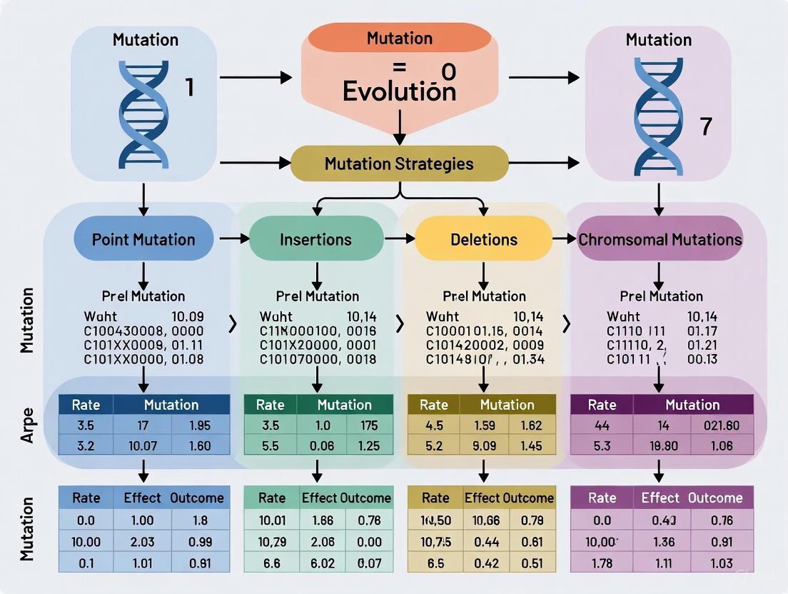
The Building Blocks of Evolution Strategies: Understanding Mutation Operators
Core Principles of Evolution Strategies versus Genetic Algorithms
Frequently Asked Questions (FAQs)
1. What is the fundamental difference between Evolution Strategies and Genetic Algorithms?
The most fundamental difference lies in how they manage the strategy parameters, such as mutation strength. Evolution Strategies (ES) often use self-adaptation, where the strategy parameters (e.g., step sizes for mutation) are encoded within each individual and evolve alongside the solution parameters [1] [2]. This allows the algorithm to dynamically adjust its search behavior. In contrast, classic Genetic Algorithms (GAs) typically rely on fixed strategy parameters set by the user at the beginning of the run and remain constant [1] [3].
2. Which algorithm should I use for optimizing real-valued parameters?
Evolution Strategies are typically the preferred choice for continuous optimization problems in real-valued search spaces [2] [4]. Their design, including the use of real-number representation and Gaussian mutation, is naturally suited for this domain. While Genetic Algorithms can be adapted for real-valued problems (using specific representations and operators), their classic form uses a discrete (often binary) representation [1] [5].
3. How does selection differ between ES and GAs?
ES traditionally use a deterministic selection scheme. After creating and evaluating λ offspring, the best μ individuals are selected to form the next generation, either from the offspring alone (μ, λ)-selection or from the combined pool of parents and offspring (μ + λ)-selection [2]. GAs, however, often use probabilistic selection methods, like roulette wheel or tournament selection, where individuals are chosen to be parents with a probability proportional to their fitness [1] [5].
4. My algorithm is converging to a sub-optimal solution. How can I prevent this?
Premature convergence is often caused by a loss of diversity in the population.
- Increase Mutation Rate/Strength: Temporarily increase the mutation operator's effect to help the population escape the local optimum [6] [7].
- Review Selection Pressure: If using a GA, ensure your selection operator is not too greedy, allowing some less-fit individuals a chance to reproduce and maintain diversity [5].
- Utilize ES Self-Adaptation: If using an ES, the self-adaptation mechanism should, in theory, automatically increase the mutation strength to explore new regions if progress stalls [2].
5. What does the notation (μ/ρ, λ)-ES mean?
This is the standard notation for describing Evolution Strategies [2]:
- μ: The number of parents in the population.
- λ: The number of offspring generated from the parents.
- ρ: The mixing number, or how many parents are used to create a single offspring through recombination.
- Comma vs. Plus:
(μ, λ)-ES means selection occurs only from the λ offspring.(μ + λ)-ES means selection occurs from the union of the μ parents and λ offspring.
Troubleshooting Guides
Issue 1: Poor Convergence Performance
Problem: Your EA is not finding satisfactory solutions, or the fitness is improving too slowly.
Diagnosis and Resolution:
Check Parameter Tuning:
- ES: For self-adaptive ES, the learning rate
τfor strategy parameters is critical. It is often recommended to set it proportional to1/√n, wherenis the problem dimension [2]. - GA: The mutation and crossover rates are key. A high mutation rate can prevent convergence, while a rate that is too low can lead to premature convergence. Adaptive mutation rates that decrease over time can help, favoring exploration first and exploitation later [7] [8].
- ES: For self-adaptive ES, the learning rate
Verify Fitness Function: Ensure your fitness function accurately reflects the problem objectives. A poorly designed fitness function can lead the search in the wrong direction.
Adjust Population Size: A population that is too small may not hold enough diversity, while one that is too large can be computationally expensive. A common heuristic in ES is to set the offspring size
λto about 7 times the parent sizeμ[4].
Issue 2: Handling Constraints in Real-Valued Optimization
Problem: Your algorithm is generating candidate solutions that violate problem constraints.
Diagnosis and Resolution:
- Penalty Functions: Incorporate a penalty term into the fitness function that reduces the fitness of infeasible solutions based on their constraint violation [2].
- Specialized Operators: Use mutation and recombination operators that are aware of and respect the variable boundaries. For example, when a mutated real value falls outside its allowed range
[x_min, x_max], it can be reflected back or set to the boundary [6]. - Repair Algorithms: Implement a procedure that takes an infeasible solution and modifies it to become feasible before fitness evaluation.
Comparative Analysis: Key Experimental Data
Table 1: Core Algorithmic Differences
| Feature | Evolution Strategies (ES) | Genetic Algorithms (GA) |
|---|---|---|
| Primary Representation | Real-valued vectors [1] [2] | Binary strings (classic) or other discrete encodings [1] [5] |
| Core Variation Operators | Mutation as the primary operator; recombination is common [2] [9] | Crossover as the primary operator; mutation is a background operator [5] [8] |
| Mutation Type | Gaussian mutation (often with self-adapting step size) [2] [6] | Bit-flip, swap, inversion, etc. [6] [7] [5] |
| Selection Method | Deterministic ((μ, λ) or (μ + λ)) [2] |
Probabilistic (e.g., roulette wheel, tournament) [1] [5] |
| Strategy Parameters | Often self-adapted [1] [2] | Typically user-defined and static [1] [3] |
Table 2: Common Mutation Operators
| Operator Name | Typical Encoding | Description | Purpose |
|---|---|---|---|
| Gaussian Mutation | Real-valued [2] [6] | Adds a random value from a Gaussian distribution to a gene. | Fine-grained local search and exploitation. |
| Bit-Flip Mutation | Binary [6] [5] | Randomly selects bits in a string and flips them (0→1, 1→0). | Introduces diversity in binary-coded populations. |
| Swap Mutation | Permutation [7] | Randomly selects two genes and swaps their positions. | Maintains diversity in combinatorial problems like scheduling. |
| Inversion Mutation | Permutation [6] [7] | Selects a substring and reverses the order of genes within it. | Creates a larger disruption to escape local optima in permutations. |
Experimental Protocol: Comparing Mutation Strategies
Objective: To empirically evaluate the performance of a self-adaptive Evolution Strategy against a canonical Genetic Algorithm on a set of continuous benchmark functions.
1. Methodology
- Benchmark Functions: Select standard functions (e.g., Sphere, Rastrigin, Ackley) with known optima to test convergence, accuracy, and robustness against local optima [2].
- Algorithm Configurations:
- ES: Implement a
(μ/μ_I, λ)-σSA-ES (where μ_I denotes intermediate recombination) [2]. - GA: Implement a real-coded GA using blend crossover (BLX-α) and Gaussian mutation.
- ES: Implement a
- Performance Metrics: Record the best fitness found over generations, the number of function evaluations to reach a target fitness, and the final solution accuracy.
2. Workflow Diagram
The following diagram illustrates the high-level workflow of a typical Evolution Strategy, highlighting the self-adaptation process.
The Scientist's Toolkit: Research Reagent Solutions
Table 3: Essential Algorithmic Components
| Item | Function | Example in ES | Example in GA |
|---|---|---|---|
| Representation Schema | Defines how a candidate solution is encoded in the algorithm. | Real-valued vector (y, σ) [2]. |
Binary string "1011001" [5]. |
| Variation Operator | Creates new candidate solutions from existing ones. | Gaussian mutation with self-adaptive step size [2] [6]. | Single-point or uniform crossover [5] [8]. |
| Selection Mechanism | Determines which solutions are allowed to reproduce. | Deterministic (μ, λ)-selection [2]. |
Fitness-proportionate (roulette wheel) selection [5]. |
| Strategy Parameter Controller | Adjusts the algorithm's internal parameters during the run. | Log-normal self-adaptation of mutation strength σ [2]. |
Predefined, static mutation probability (e.g., 0.01) [5]. |
In Evolution Strategies (ES), a subclass of evolutionary algorithms, mutation operators are a fundamental genetic operator that introduces random variations into a population of candidate solutions, enabling the exploration of the search space [10]. The self-adaptation of mutation step sizes is a defining feature of ES, allowing the algorithm to dynamically adjust the magnitude of perturbations during the search process [10]. Mutation operators are broadly categorized based on how these step sizes are controlled. In its simplest form, a single step size control parameter may be used for all dimensions of the search space. More advanced strategies employ uncorrelated mutations with multiple step sizes, one for each coordinate, or correlated mutations, where a full covariance matrix adapts the mutation distribution, allowing it to align with the topology of the objective function [10]. Understanding this taxonomy is crucial for researchers and practitioners applying ES to complex optimization problems in fields like drug design and protein engineering, where navigating high-dimensional, rugged search spaces efficiently is paramount.
Core Taxonomy and Definitions
The following table outlines the core characteristics, mechanisms, and typical use cases for the different classes of mutation operators in Evolution Strategies.
| Feature | Uncorrelated Mutation (Single Step Size) | Uncorrelated Mutation (n Step Sizes) | Correlated Mutation |
|---|---|---|---|
| Core Concept | A single step size parameter controls mutation for all coordinates. | Each coordinate (dimension) has its own independently adaptable step size. | Step sizes and rotations are adapted using a covariance matrix, modeling dependencies between dimensions. |
| Number of Strategy Parameters | 1 | n | n(n+1)/2 |
| Mutation Distribution | Isotropic (spherical) | Axis-parallel ellipsoidal | General ellipsoidal (can be rotated) |
| Adaptation Mechanism | Self-adaptation or derandomized methods like CMA-ES. | Self-adaptation, where each step size is mutated independently. | Covariance Matrix Adaptation (CMA), which learns the underlying correlation structure of the search space. |
| Advantages | Simple, low computational cost. | Can scale mutations differently for each axis, good for separable functions. | Can handle non-separable and ill-conditioned problems effectively by learning the search direction. |
| Disadvantages | Inefficient on functions that are not axis-aligned or are ill-conditioned. | Cannot handle correlations between parameters; performance degrades on non-separable problems. | Higher computational and memory complexity due to the covariance matrix update and decomposition. |
| Typical Application | Simple, low-dimensional optimization problems. | Medium-dimensional problems where parameters are roughly independent. | Complex, high-dimensional, non-separable optimization problems. |
Frequently Asked Questions (FAQs)
Q1: My Evolution Strategy is converging prematurely to a suboptimal solution. What could be the cause and how can I troubleshoot this?
A: Premature convergence is often a result of a poor balance between exploration and exploitation, frequently linked to the mutation operator [11].
- Check Mutation Step-Sizes: If the step-sizes have become too small too quickly, the population loses diversity and gets trapped. Inspect the log of your strategy parameters.
- Troubleshooting Action: Consider switching from a
(μ + λ)-selection strategy to a(μ, λ)-strategy. The(μ, λ)-strategy, which selects parents only from the offspring, is more effective at avoiding premature convergence because it allows for the continual renewal of the population and forgets the parent information [10]. - Troubleshooting Action: Implement a mutation operator that better maintains population diversity. Operators like Non-uniform Mutation (NUM) or Power Mutation (PM) can help by providing a more dynamic search behavior, preventing the algorithm from stagnating [11].
Q2: How do I choose between uncorrelated and correlated mutations for my specific optimization problem in drug design?
A: The choice hinges on the problem's dimensionality, complexity, and your computational budget.
- For Low-Dimensional Problems or Initial Screening: Start with an uncorrelated mutation with n step-sizes. This is computationally cheaper and can be sufficient for problems where the parameters (e.g., molecular descriptors) have minimal complex interactions [10].
- For High-Dimensional, Complex Landscapes: If you are optimizing a molecular structure where parameters are highly interdependent (a non-separable problem), correlated mutations are strongly recommended. Techniques like the Covariance Matrix Adaptation Evolution Strategy (CMA-ES) are designed to learn these interactions, significantly improving search efficiency [10]. This is analogous to structure-guided drug design, where understanding the relationship between a protein's structure and function is key to designing effective inhibitors [12].
Q3: In a real-coded Genetic Algorithm (GA), my crossover operator seems to be causing unstable solutions with high variance. What's wrong?
A: This is a common challenge where conventional crossover operators fail to maintain a proper balance between exploration and exploitation, especially in multimodal and high-dimensional problems [11].
- Troubleshooting Action: Evaluate your current crossover operator. Standard operators like Simulated Binary Crossover (SBX) or Laplace Crossover (LX) may struggle with population diversity and adaptation.
- Troubleshooting Action: Consider implementing more robust, parent-centric real-coded crossover operators. Recent research has proposed operators like Mixture-based Gumbel Crossover (MGGX) and Mixture-based Rayleigh Crossover (MRRX), which are designed to dynamically adapt and generate diverse yet high-quality offspring. Studies show that MGGX, in particular, can achieve lower mean and standard deviation values, indicating more stable and reliable performance across various benchmark functions [11].
Experimental Protocols for Mutation Analysis
Protocol: Benchmarking Mutation Operator Performance
This protocol provides a standardized methodology for comparing the efficacy of different mutation operators, such as uncorrelated versus correlated, within an Evolution Strategy.
1. Objective: To quantitatively assess and compare the performance of different mutation operators on a set of standardized optimization problems. 2. Materials (Software & Computational Environment):
- Programming Language: Python (with libraries like NumPy and SciPy) or C++.
- ES Framework: A custom implementation or a library like
cma-es(for CMA-ES) in Python. - Computing Platform: A standard workstation or high-performance computing cluster for more demanding tests.
3. Methodology:
- Step 1: Selection of Benchmark Functions. Choose a diverse set of functions with known properties:
- Unimodal Function: e.g., Sphere (to measure pure convergence speed).
- Multimodal Function: e.g., Rastrigin (to test ability to escape local optima).
- Ill-Conditioned/Non-separable Function: e.g., Ellipsoid or Cigar (to test the need for correlated mutations).
- Step 2: Algorithm Configuration.
- Implement the ES with the mutation operators under test (e.g., uncorrelated with one step-size, uncorrelated with n step-sizes, and correlated via CMA).
- Keep all other parameters constant: population size (μ and λ), recombination method, and initial solution. A common setting is
(μ, λ)-selection with μ = λ/2 [10]. - For self-adaptation, use the standard log-normal update rule for step-sizes:
σ_j' = σ_j * exp(τ * N(0,1))[10].
- Step 3: Data Collection and Metrics.
- Run each (mutation operator, benchmark function) combination multiple times (e.g., 50 independent runs) to account for stochasticity.
- Record for each run:
- Best Fitness vs. Generation: To plot learning curves.
- Final Solution Quality: The best objective value found.
- Number of Function Evaluations to reach a target fitness.
- Step 4: Statistical Analysis.
- For each function, calculate the mean and standard deviation of the final solution quality across all runs for each operator [11].
- Perform statistical significance tests (e.g., Wilcoxon signed-rank test) to confirm that performance differences are not due to chance.
- Use multi-criteria decision-making methods like TOPSIS or the Quade test to rank the overall performance of the operators across all benchmark functions [11].
- Step 1: Selection of Benchmark Functions. Choose a diverse set of functions with known properties:
Protocol: Self-Adaptation of Mutation Step-Sizes
This protocol details the core mechanism of how strategy parameters (step-sizes) are mutated in a self-adaptive Evolution Strategy.
1. Objective: To implement and observe the self-adaptation process of mutation step-sizes in an uncorrelated mutation operator with n step-sizes.
2. Methodology:
* Step 1: Representation. Each individual in the population is a tuple a = (x, σ), where x is the object variable vector (the solution) and σ is the vector of n step-sizes, one for each dimension in x.
* Step 2: Mutation of Strategy Parameters. The step-size vector σ is mutated before the solution vector x. This is a critical aspect of self-adaptation.
* For each dimension j in σ, update the step-size:
σ_j' = σ_j * exp(τ * N(0,1)) ...(Global factor)
* A more common and effective method is to also include an independent perturbation for each dimension:
σ_j' = σ_j * exp(τ * N(0,1) + τ' * N_j(0,1)) ...(Global and individual factors)
* Here, N(0,1) is a standard normal random number drawn once for the entire individual, and N_j(0,1) is a new number drawn for each dimension j. The learning rates τ and τ' are pre-defined constants.
* Step 3: Mutation of Object Variables. After the new step-sizes σ' are computed, the solution vector x is mutated.
* For each dimension j in x:
x_j' = x_j + σ_j' * N_j(0,1)
* The mutation of x uses the newly mutated step-sizes σ_j', ensuring that offspring which inherit "good" step-sizes are more likely to survive [10].
Visualizing Mutation Strategies and Workflows
Mutation Strategy Decision Workflow
The diagram below outlines a logical workflow for selecting an appropriate mutation strategy based on problem characteristics.
Self-Adaptation Mechanism
This diagram illustrates the process flow for the self-adaptation of mutation step-sizes, a core concept in Evolution Strategies.
The Scientist's Toolkit: Essential Research Reagents & Algorithms
The following table details key algorithms, components, and computational "reagents" essential for experimentation with mutation operators in Evolution Strategies.
| Item Name | Type | Function / Application |
|---|---|---|
| CMA-ES Algorithm | Algorithm | A state-of-the-art Evolution Strategy that uses correlated mutations by adapting a full covariance matrix. Ideal for complex, non-separable optimization problems [10]. |
| Benchmark Function Suite | Software Tool | A collection of standard optimization problems (e.g., Sphere, Rastrigin, Cigar) used to rigorously test and compare the performance of different algorithms and operators [11]. |
| Real-Coded Genetic Algorithm (GA) | Algorithm Framework | A population-based optimization algorithm that works directly with real-valued parameters. Serves as a testbed for integrating and evaluating new crossover and mutation operators [11]. |
| MGGX / MRRX Crossover | Crossover Operator | Novel, parent-centric real-coded crossover operators designed to dynamically balance exploration and exploitation, often outperforming conventional operators like SBX in complex scenarios [11]. |
| Non-Uniform Mutation (NUM) | Mutation Operator | A mutation operator commonly used in GAs where the magnitude of mutation decreases over time, helping to shift from global exploration to local exploitation as the run progresses [11]. |
| Power Mutation (PM) | Mutation Operator | A mutation operator based on the power distribution, used to increase population diversity and help the algorithm escape local optima [11]. |
| Covariance Matrix | Data Structure | An n×n matrix at the heart of correlated mutations. It is adapted over generations to model the pairwise dependencies between decision variables, shaping the mutation distribution [10]. |
| Selection Strategies ((μ,λ) vs (μ+λ)) | Algorithmic Rule | Determines how the parent population for the next generation is formed. The (μ,λ) strategy often helps prevent premature convergence [10]. |
This technical support center provides troubleshooting guides and FAQs for researchers working with Evolution Strategies (ES). The content is framed within a broader thesis comparing mutation strategies, assisting scientists in diagnosing and resolving common issues with strategy parameters.
Frequently Asked Questions (FAQs)
1. My (μ/μ,λ)-ES is converging prematurely. How can I adjust the strategy parameters to improve exploration? Premature convergence often indicates a loss of population diversity and insufficient exploration. The following adjustments are recommended:
- Increase the Offspring Population Size (λ): Using a larger λ relative to the parent population size (μ) promotes exploration. A common heuristic is to set λ = 7μ [4].
- Re-evaluate the Step-Size (σ) Adaptation Rule: If you are using a simple rule like the 1/5th success rule, ensure it is functioning correctly. This rule states that you should decrease the mutation step size if the success rate (the fraction of mutations that lead to an improvement) is below 1/5, and increase it if it is above [13] [4]. A success rate consistently below 1/5 may require a larger base step size.
- Consider a Different Mutation Strategy: Switch from a strategy that heavily exploits the best solution (e.g., "best" based) to one that emphasizes exploration, such as "rand" based strategies which use randomly selected individuals [14].
2. My CMA-ES algorithm is running slowly on a high-dimensional problem. What steps can I take to improve its efficiency? Performance issues in high dimensions are often related to the complexity of updating the covariance matrix.
- Algorithm Selection: For very high-dimensional problems (e.g., >1000 parameters), consider using a variant like the Limited-Memory CMA-ES (L-CMA-ES), which reduces time and memory complexity by using a compressed representation of the covariance matrix [10].
- Parallelization: ES are highly amenable to parallelization. You can significantly speed up the fitness evaluation step by distributing the evaluation of offspring across multiple CPU cores [15]. The forward-pass-only nature of ES makes this more efficient than gradient-based methods that require backpropagation.
- Check Hyperparameters: Review the learning rates for the evolution paths and covariance matrix update (e.g., αcλ, αc1). The default settings are usually robust, but for specific problem landscapes, tuning may be necessary [16].
3. How do I choose between the (μ,λ) and (μ+λ) selection strategies? The choice fundamentally trades off exploration for convergence speed and robustness.
- Use (μ,λ)-ES: This strategy selects the next generation parents only from the newly created λ offspring. It does not include the previous parents. This is better for exploration and is more robust in dynamic environments or when dealing with noisy fitness functions, as it can "forget" bad parents [10] [4].
- Use (μ+λ)-ES: This strategy selects the next generation parents from the combined pool of the μ parents and λ offspring. This is an elitist strategy that guarantees the best solution found so far is never lost. It typically leads to faster convergence but may be more prone to getting stuck in local optima [10] [4].
Heuristic: A common and robust setting is to use the (μ,λ) strategy with λ = 7μ [4].
Troubleshooting Guides
Problem: Ineffective Step-Size Adaptation
Symptoms:
- The algorithm stagnates, showing no improvement over many generations.
- The step-size (σ) collapses to zero, halting all exploration.
- Oscillating performance where the step-size repeatedly grows too large and then shrinks too small.
Diagnosis and Solutions: This problem arises when the step-size adaptation mechanism is not correctly aligned with the local fitness landscape.
Verify the 1/5th Success Rule Implementation:
- Protocol: Calculate the success rate over a sliding window of the last n iterations, where n is the problem dimensionality [13].
- Action: Adjust the step-size multiplicatively based on the measured success rate (ps):
- If ps < 1/5: Set σ = σ * c (e.g., c = 0.85)
- If ps > 1/5: Set σ = σ / c
- Rationale: This rule ensures that the step-size is reduced to fine-tune solutions when progress is hard to find, and increased to take larger steps when progress is easy [13] [4].
Inspect Evolution Paths in CMA-ES:
- Concept: In CMA-ES, the step-size is adapted using an evolution path—a weighted history of the movement of the population mean. A short path indicates cancelling steps (step-size too large), while a long, straight path indicates consistent progress (step-size could be increased) [16].
- Visualization: The following diagram illustrates the step-size adaptation logic in CMA-ES based on the evolution path length.
- Action: If the step-size is not adapting well, check the update rule for the evolution path pσ. The damping parameter dσ controls the step-size change magnitude [16].
Problem: Poor Convergence Rate on Ill-Conditioned Problems
Symptoms:
- Slow progress along specific dimensions of the search space.
- Performance is significantly worse on non-separable, ill-conditioned functions compared to spherical functions.
Diagnosis and Solutions: The algorithm is failing to learn and exploit the structure of the fitness landscape, specifically the scaling of and correlations between variables.
- Switch to CMA-ES:
- Rationale: The Covariance Matrix Adaptation Evolution Strategy (CMA-ES) is specifically designed to address this issue. It automatically adapts a full covariance matrix of the mutation distribution, which effectively models the dependencies between variables [10] [16].
- Protocol:
- Initialization: Initialize the mean vector (μ), step-size (σ), and covariance matrix (C = I).
- Mutation: Generate λ offspring: xi = μ + σ * yi, where y_i ~ N(0, C).
- Selection and Recombination: Update the mean μ by taking a weighted average of the best-performing offspring.
- Covariance Matrix Adaptation: Update the covariance matrix C using information from both the current generation's best offspring and the long-term evolution path [16].
- Visualization: The workflow of the CMA-ES algorithm is outlined below.
- Check for Parameter Misconfiguration:
- Population Size: A larger population size (λ) can help in building a more reliable estimate of the covariance matrix, especially in higher dimensions. Consider using an increased population size [17].
- Learning Rates: The default learning rates for the covariance matrix update (e.g., αc1 for the rank-one update) are typically well-chosen. Modifying them without deep understanding of the algorithm can be detrimental [16].
Comparative Data Tables
Table 1: Comparison of Common Mutation Strategy Parameterizations
| Strategy | Parameters Controlled | Adaptation Mechanism | Best For |
|---|---|---|---|
| Isotropic Gaussian (1+1)-ES | Single step-size (σ) | 1/5th Success Rule [13] [4] | Simple, convex problems; quick prototyping. |
| Derandomized Self-Adaptation | n step-sizes (σ₁,...,σₙ) | Log-normal self-adaptation [10] | Problems with separable variables and different sensitivities per dimension. |
| CMA-ES | Full covariance matrix (C) & step-size (σ) | Evolution paths and rank-μ/rank-one updates [10] [16] | Non-separable, ill-conditioned, and rugged problems. |
Table 2: Performance Comparison of Selection Schemes
| Selection Scheme | Convergence Speed | Robustness to Noise | Risk of Premature Convergence |
|---|---|---|---|
| (1+1) | Fast (on simple problems) | Low | High |
| (μ+λ) | Fast | Medium | Medium-High |
| (μ,λ) | Slower | High | Low |
The Scientist's Toolkit: Essential Research Reagents
Table 3: Key Algorithmic Components and Their Functions
| Component | Function | Example in ES Context |
|---|---|---|
| Mutation Strength (σ) | Controls the global scale of exploration in parameter space. A larger σ enables larger jumps [16] [4]. | The step-size in Simple Gaussian ES. |
| Covariance Matrix (C) | Encodes the shape and orientation of the mutation distribution, modeling variable dependencies and scaling [16]. | The adaptive matrix in CMA-ES that replaces the identity matrix. |
| Evolution Path | Tracks the direction of successful mutations over multiple generations, allowing for cumulative step-size adaptation [16]. | The path pσ used in CMA-ES to decide whether to increase or decrease σ. |
| Recombination Weights | Assigns different importance to selected parents when creating a new mean, typically favoring better individuals [16]. | The weights used in (μ/μ,λ)-ES to update the population mean. |
| Success Rule | A heuristic to adapt strategy parameters based on the observed frequency of successful mutations [13]. | The 1/5th rule for step-size control. |
This guide supports a broader thesis comparing mutation strategies in Evolution Strategies (ES) research. For researchers in fields like drug development, where model parameters must be finely tuned amidst noisy data, understanding and troubleshooting self-adaptation mechanisms—how an algorithm automatically controls its own mutation strength—is crucial for achieving robust performance. This resource provides targeted FAQs and experimental protocols to address specific issues encountered during implementation.
Frequently Asked Questions (FAQs) and Troubleshooting
FAQ 1: Why does my self-adaptive ES converge prematurely to a suboptimal solution?
- Problem: This is often due to mutation strength collapse, where the step-size parameter (σ) decreases too rapidly, halting exploration before finding the global optimum [18].
- Solution:
- Check Learning Parameters: The primary learning parameter
τ(tau) may be too large, causing excessive selection pressure on smaller step-sizes. Try reducingτ; a rule of thumb is τ ∝ 1/√n, where n is the number of parameters [18]. - Verify Sampling Method: Log-normal sampling (
σ_SAL) inherently introduces a bias towards larger step-sizes under random selection. If your population size is small, this bias can be detrimental. Consider switching to unbiased normal sampling (σ_SAN), whereσ_SAN = σ * (1 + τ * N(0,1))[18]. - Increase Population Size: A larger population (
μ,λ) helps maintain genetic diversity, providing more information for the self-adaptation mechanism to correctly adjust σ [18].
- Check Learning Parameters: The primary learning parameter
FAQ 2: How do I choose between Cumulative Step-size Adaptation (CSA) and Mutative Self-Adaptation (σSA)?
- Problem: Uncertainty about which σ-control mechanism is better suited for a specific problem type.
- Solution: The choice depends on the problem landscape and computational resources. The table below summarizes the key characteristics based on recent research [18]:
Table: Comparison of σ-Control Mechanisms
| Feature | Cumulative Step-size Adaptation (CSA) | Mutative Self-Adaptation (σSA) |
|---|---|---|
| Core Principle | Uses an evolution path to adapt σ based on the consistency of successful directions [18]. | Selects σ values based on the fitness of the offspring they produce [18]. |
| Adaptation Speed | Can be slower, especially with large populations [18]. | Can achieve faster adaptation and larger progress rates [18]. |
| Typical Use Case | Well-suited for noisy optimization problems [18]. | Effective on complex, multimodal fitness landscapes. |
| Parameter Sensitivity | Requires tuning of cumulation and damping parameters [18]. | Sensitive to the learning parameter τ [18]. |
FAQ 3: My algorithm's performance is highly variable between runs. What is wrong?
- Problem: High performance variance often stems from poor parameter settings or an incorrectly configured self-adaptation workflow.
- Solution:
- Re-examine the Workflow: Ensure your implementation correctly follows the self-adaptation logic. The diagram below outlines the core process for a (μ/μ_I, λ)-σSA-ES.
- Conduct Parameter Sensitivity Analysis: Systematically test different values for
τ,μ, andλon a simple benchmark function like the sphere model to understand their impact [18]. - Inspect the σ Path: Log the value of σ over generations. A healthy run should show σ adapting dynamically rather than monotonically decreasing or increasing.
Self-Adaptation Workflow in a (μ/μ_I, λ)-σSA-ES
Experimental Protocols and Methodologies
To validate and compare the performance of different self-adaptation mechanisms, the following experimental protocols are recommended.
Protocol 1: Benchmarking on the Sphere Model
The sphere model is a standard test function to analyze the core properties of ES, defined as f(x) = Σx_i² [18].
- Algorithm Setup: Implement a (μ/μ_I, λ)-ES with both σSA and CSA.
- Parameter Normalization: Use normalized progress rate (φ) and normalized mutation strength (σ) for scale-invariant analysis: φ* = φN/R and σ* = σN/R [18].
- Measurement: Run the ES for a fixed number of generations and record:
- The progress rate φ* over time.
- The steady-state level of σ*.
- The number of generations to reach a predefined fitness threshold.
- Analysis: Compare the adaptation speed and stability of σ* between σSA and CSA. The theoretical progress rate for the sphere can be used as a baseline for validation [18].
Protocol 2: Analyzing Adaptation on a Multimodal Function
Use a function like the Rastrigin function, which has many local optima, to test the global search capabilities and avoidance of premature convergence [19].
- Setup: Initialize the population far from the global optimum.
- Observation: Monitor how the mutation strength σ changes when the population encounters a local optimum. A well-adapted ES should temporarily increase σ to escape the basin of attraction.
- Metric: Record the success rate of finding the global optimum over multiple independent runs.
Research Reagent Solutions
The table below details the key algorithmic components required for implementing and experimenting with self-adaptive Evolution Strategies.
Table: Essential Components for Self-Adaptive ES Research
| Research Reagent | Function & Description |
|---|---|
| Mutation Sampling Scheme | Defines how offspring mutation strengths are generated. The two primary types are Log-Normal (biased) and Normal (unbiased), crucially impacting adaptation [18]. |
| Recombination Operator | The method for creating the new parental σ from selected offspring σ' values. Intermediate recombination is common in (μ/μ_I, λ)-ES [18]. |
| Learning Parameter (τ) | Controls the magnitude of changes in the mutation strength during sampling. It is a critical parameter that often requires problem-specific tuning [18]. |
| Population Size (μ, λ) | The number of parent (μ) and offspring (λ) individuals. Larger populations provide more information for reliable self-adaptation but increase computational cost [18]. |
| Fitness Benchmark Suite | A set of test functions (e.g., Sphere, Rastrigin, Schaffer) used to evaluate and compare the performance and robustness of different algorithm configurations [19] [18]. |
Implementing Mutation Strategies: From Theory to Biomedical Applications
Frequently Asked Questions
Q1: Why is my ES population converging prematurely to a suboptimal solution?
Premature convergence often occurs due to a loss of genetic diversity, frequently caused by an incorrectly calibrated mutation strength. If the mutation step size is too small, the algorithm cannot escape local optima [4]. To remedy this, ensure you are using a sufficiently large population size and adapt your mutation strength dynamically using rules like the 1/5th success rule or self-adaptation strategies where strategy parameters evolve alongside the solution parameters [4] [20].
Q2: How do I choose between the (μ, λ)-ES and (μ + λ)-ES selection strategies?
The choice impacts the algorithm's explorative character. Use the comma-selection (μ, λ)-ES for dynamic problems or when you need to maintain strong exploration pressure, as it discards parents entirely. Use the plus-selection (μ + λ)-ES for refining solutions and converging more reliably on static problems, as it allows parents to compete for survival [20]. A common heuristic is to set λ = 7μ [4].
Q3: What is the purpose of mutating strategy parameters?
Mutating strategy parameters—like the step size in Gaussian mutation—allows the algorithm to self-adapt to the local topology of the search landscape. This co-evolution of solution and strategy parameters enables the algorithm to automatically adjust the magnitude of its mutations, balancing exploration and exploitation without manual intervention [20].
Q4: My mutation operator is generating solutions that violate constraints. How can I fix this?
For simple box constraints, a direct approach is to clamp the values to the feasible range after mutation [20]. For more complex constraints, you may need to incorporate constraint-handling techniques such as penalty functions or repair mechanisms into your fitness evaluation. The mutation operators themselves can also be designed to be aware of the value range of decision variables [6].
Troubleshooting Guides
Problem: Slow or Stagnant Convergence Possible Causes and Solutions:
- Cause: Inadequate mutation strength.
- Cause: Insufficient population diversity.
- Solution: Increase the ratio of offspring to parents (
λ / μ). A larger population size (μ) can also improve exploration [4].
- Solution: Increase the ratio of offspring to parents (
- Cause: The recombination operator is causing premature homogenization.
- Solution: Experiment with different recombination operators. For instance, discrete recombination (randomly selecting parameters from parents) can promote more diversity than intermediate recombination (averaging parent parameters) [4].
Problem: Algorithm is Too Noisy and Fails to Refine Solutions Possible Causes and Solutions:
- Cause: Mutation strength is too high, causing the algorithm to behave like a random search.
- Solution: Decrease the initial mutation step size and use a plus-selection strategy
(μ + λ)-ESto better preserve good solutions [20].
- Solution: Decrease the initial mutation step size and use a plus-selection strategy
- Cause: The population size is too large for the available computational budget.
- Solution: While a larger population aids exploration, it requires more function evaluations. You may need to reduce the population size or offspring count and run the algorithm for more generations [4].
Experimental Protocols and Data Presentation
Table 1: Common Mutation Operators for Different Encodings
| Genome Type | Suitable Mutation Operators | Key Characteristics | Applicability in Drug Development |
|---|---|---|---|
| Real-Valued | Gaussian Mutation [6] [20] | Adds noise from a normal distribution; small steps are more likely. | Optimizing continuous parameters like molecular docking coordinates or chemical concentration ratios. |
| Uniform Mutation [6] | Replaces a value with a random one from a uniform distribution. | Exploring a wide range of possible values, such as in initial screening phases. | |
| Binary String | Bit Flip Mutation [6] | Flips individual bits (0 becomes 1, and vice versa) at random positions. | Optimizing feature selection masks in QSAR (Quantitative Structure-Activity Relationship) models. |
| Permutations | Inversion [6] | Reverses the order of a randomly selected subsequence. | Scheduling the order of laboratory experiments or synthetic steps. |
| Insertion/Deletion/Swap [6] | Moves, deletes, or swaps elements within the sequence. | Designing peptide sequences or optimizing molecular structures represented as sequences. |
Table 2: Key Strategy Parameters and Performance Heuristics
| Parameter | Description | Heuristic & Impact |
|---|---|---|
| Population Size (μ) | Number of parent solutions in each generation. | A larger μ improves exploration but increases computational cost [4]. |
| Offspring Count (λ) | Number of new solutions created each generation. | Typically λ > μ; a common setting is λ = 7μ to promote diversity [4]. |
| Mutation Strength (σ) | Standard deviation for Gaussian mutation. | Should be adapted; can be initialized as (x_max - x_min)/6 [6]. The 1/5th success rule is a classic adaptation heuristic [20]. |
| Recombination Size (ρ) | Number of parents used to create one offspring. | Often set to ρ = 2 for intermediate recombination; can be higher for discrete recombination [4]. |
Detailed Methodology: Gaussian Mutation with Self-Adaptation
This is a common and powerful protocol for continuous optimization problems [20].
- Representation: Each individual in the population is represented as a tuple
(x, σ), wherexis the vector of decision variables (e.g., molecular descriptors) andσis a vector of strategy parameters (step sizes) for each dimension. - Mutation of Strategy Parameters: First, mutate the step sizes for each offspring:
σ_i' = σ_i * exp(τ' * N(0,1) + τ * N_i(0,1))- Here,
N(0,1)is a standard normal random variable, sampled once for alli, andN_i(0,1)is sampled anew for eachi. The learning ratesτandτ'are set asτ ∝ 1/√(2n)andτ' ∝ 1/√(2√n), wherenis the problem dimension [20].
- Mutation of Object Variables: Then, mutate the solution itself using the new step sizes:
x_i' = x_i + σ_i' * N_i(0,1)
- Selection and Iteration: Evaluate the fitness of the new offspring
(x', σ')and proceed with selection (e.g.,(μ, λ)-selection) to form the next generation.
Workflow and Strategy Visualization
The Scientist's Toolkit: Essential Research Reagents
Table 3: Key Research Reagent Solutions for ES Experiments
| Item | Function in ES Research | Example & Notes |
|---|---|---|
| Optimization Framework | Provides the foundational algorithms and operators. | Examples: DEAP (Python), JMetal, HeuristicLab. These libraries offer implemented ES variants, mutation operators, and benchmarking tools. |
| Benchmark Problem Set | Standardized functions to validate and compare algorithm performance. | Examples: BBOB (Black-Box Optimization Benchmarking), Noisy Test Problems. Used to test convergence, robustness, and scalability of a new mutation strategy [20]. |
| Step-Size Adaptation Rule | A heuristic or mechanism to control mutation strength. | Examples: The 1/5th Success Rule, Log-Normal Self-Adaptation, CMA-ES. Critical for automating the tuning of the mutation operator [4] [20]. |
| Statistical Analysis Tool | For rigorous comparison of experimental results. | Examples: R, Python (with SciPy/statsmodels). Used to perform significance tests (e.g., Wilcoxon signed-rank test) on results from multiple independent runs. |
Model-Informed Drug Development (MIDD) is a quantitative framework that uses modeling and simulation to inform drug development decisions and regulatory evaluations. It encompasses a range of methodologies, including Quantitative Systems Pharmacology (QSP), which uses mechanistic models to simulate drug effects within biological systems [21] [22]. Within a research thesis comparing mutation strategies, these models act as sophisticated "fitness functions," where in silico simulations help identify optimal drug candidates and parameters before costly real-world experiments, mirroring how evolutionary algorithms search for optimal solutions [23].
This guide provides technical support for applying these approaches, with troubleshooting focused on common challenges in model development and validation.
Troubleshooting Guides
Problem 1: Poor Model Performance or Lack of Predictive Power
Issue: Your QSP or MIDD model fails to accurately predict experimental or clinical outcomes.
Diagnosis and Solutions:
| Diagnostic Step | Potential Root Cause | Recommended Action |
|---|---|---|
| Parameter Evaluation | Poorly constrained or inaccurate parameters [24]. | Perform global sensitivity analysis to identify most influential parameters. Focus calibration efforts on these [25]. |
| Model Structure Check | Oversimplified biology or missing key pathways [21]. | Review latest literature and omics data to ensure critical mechanisms are included. Consider a more granular semi-mechanistic approach [21]. |
| Data Integration Review | Inadequate or poor-quality data for model training/validation [24]. | Use AI-driven data imputation or synthetic data generation to fill gaps. Prioritize collecting high-quality, targeted data [24]. |
| Validation Method | Reliance on single, non-representative validation dataset [25]. | Employ a Virtual Population (VP) approach. Generate many in silico patients and confirm predictions hold across this population [25]. |
Experimental Protocol: Virtual Population (VP) Analysis for Model Validation
- Objective: To quantify the robustness of a qualitative model prediction (e.g., "Drug A is superior to Drug B").
- Methodology:
- Generate Virtual Subjects: Create a large cohort (e.g., 1,000-10,000) of in silico patients by sampling model parameters from predefined physiological distributions [25].
- Run Simulations: Execute your model for each virtual subject in the cohort for each scenario (e.g., Drug A vs. Drug B).
- Calculate Prediction Distribution: For each subject, calculate the outcome metric (e.g., % tumor shrinkage). Determine the percentage of the virtual population for which the qualitative prediction holds true (e.g., % of patients where Drug A outperforms Drug B).
- Statistical Testing: Compare this distribution against a null hypothesis (e.g., from random parameter sets or random "drugging" of proteins) using appropriate statistical tests (e.g., Chi-squared) to assess significance [25].
Problem 2: Model is Too Slow for Practical Use
Issue: Simulations, especially large-scale virtual population or parameter exploration runs, take too long, hindering iterative development.
Diagnosis and Solutions:
| Diagnostic Step | Potential Root Cause | Recommended Action |
|---|---|---|
| Code Profiling | Inefficient algorithms or coding practices. | Use profiling tools to identify computational bottlenecks. Refactor critical sections of code. |
| Platform Assessment | Hardware limitations (e.g., local machine). | Migrate to cloud-based computational platforms designed for large-scale QSP simulations [26]. |
| Model Complexity | Unnecessarily high model resolution for the COU. | Implement a "Fit-for-Purpose" strategy. Simplify the model where possible without compromising key outputs [21]. Use declarative programming environments that optimize execution [26]. |
Issue: The model cannot effectively incorporate or reconcile data from different sources (e.g., in vitro, omics, clinical trials).
Diagnosis and Solutions:
| Diagnostic Step | Potential Root Cause | Recommended Action |
|---|---|---|
| Data Audit | Incompatible formats, scales, or missing metadata. | Implement a unified data infrastructure or use AI-powered platforms to harmonize and integrate diverse datasets [24]. |
| Workflow Review | Manual, error-prone data processing pipelines. | Adopt end-to-end QSP platforms with built-in data handling and curation tools to streamline workflows [26]. |
Frequently Asked Questions (FAQs)
Q1: What is the difference between a "top-down" (e.g., PopPK) and "bottom-up" (e.g., QSP) MIDD approach, and when should I use each?
A1: The choice is dictated by the "Question of Interest" (QOI) and available data [21] [22].
- Top-Down (e.g., PopPK, PK/PD): These are primarily data-driven. They analyze observed clinical data to describe what happens (e.g., quantifying dose-exposure-response and identifying sources of variability). Use them when you have rich clinical data and need to describe relationships and variability in a population [22].
- Bottom-Up (e.g., QSP, PBPK): These are primarily mechanism-driven. They build on prior knowledge of physiology and biology to simulate how it happens. Use them for prospective prediction in data-sparse environments (e.g., first-in-human dose), understanding biological mechanisms, or optimizing combination therapies [22].
Q2: How do I know if my QSP model is "validated," especially since it has many unidentifiable parameters?
A2: Validation for QSP differs from traditional PK/PD models. Shift focus from "parameter identifiability" to "prediction credibility" [25].
- Qualitative Prediction: Can the model reproduce known, non-fitted biological behaviors or clinical outcomes? [25]
- Virtual Population (VP) Analysis: As described in the troubleshooting guide, use VPs to generate a distribution of predictions and test the robustness of qualitative findings [25].
- Biological Plausibility: The model's structure and dynamics should be reviewed and accepted by domain experts for biological realism [25].
Q3: Our QSP models are built by a single expert, creating a bottleneck. How can we make QSP more scalable and accessible?
A3: This is a common challenge driven by model complexity and reliance on specialized coding skills [26]. Solutions include:
- Utilize Pre-validated Model Libraries: Start from existing, documented models for common therapeutic areas to reduce development time [26].
- Adopt Democratizing Platforms: Use platforms with intuitive, visual interfaces and declarative programming that reduce the coding burden for non-specialists [26].
- Implement Collaboration Tools: Use software with features that allow teams to share, edit, and compare models and scenarios, breaking down knowledge silos [26].
Q4: How is AI being used to supercharge traditional QSP modeling?
A4: AI and machine learning are being integrated to address key limitations [24]:
- Data Gap Filling: AI can generate robust synthetic data to impute missing biological parameters (e.g., target expression levels) [24].
- Automated Parameterization: ML algorithms (e.g., Bayesian inference) can automate and accelerate model parameter estimation and calibration [24].
- Enhanced Predictive Capability: AI can help build models that better capture inter-individual variability, enabling more reliable virtual trials and patient stratification [24].
The Scientist's Toolkit: Research Reagent Solutions
| Tool / Reagent | Function in MIDD/QSP | Key Consideration |
|---|---|---|
| PBPK Platform (e.g., GastroPlus, Simcyp) | Mechanistically simulates ADME and predicts human PK, DDI, and dosing in special populations [22]. | Quality of system-specific (physiological) and drug-specific (input) parameters is critical for reliable predictions. |
| QSP Software (e.g., Certara IQ, BIOiSIM) | Provides environment to build, simulate, and analyze complex QSP models; some offer AI-enhanced features and model libraries [26] [24]. | Choose based on usability, computational speed, and availability of models relevant to your therapeutic area. |
| PopPK/PD Software (e.g., NONMEM, Monolix) | Performs nonlinear mixed-effects modeling to quantify population mean parameters and inter-individual variability [21]. | Requires expertise in model coding, diagnostics, and statistical interpretation. |
| Model-Based Meta-Analysis (MBMA) | Uses curated historical clinical trial data for indirect comparison to competitors and optimization of trial design [22]. | The quality and breadth of the underlying database are paramount. |
| Virtual Population Generator | Creates in silico cohorts of virtual patients for simulating variability and quantifying uncertainty in predictions [25]. | The method for generating the population (e.g., stochastic search, sampling) can influence results. |
Detailed Experimental Protocol: QSP for Combination Therapy Scheduling
This protocol outlines how a QSP model can be used to identify an optimal dosing schedule for a combination therapy, a common and challenging application.
- Background: Drug combinations can show schedule-dependent effects where the sequence of administration impacts overall efficacy or safety [25].
- Objective: To use a calibrated QSP model of cancer cell signaling and proliferation to simulate and compare the efficacy of different dosing sequences for Gemcitabine and Birinapant [25].
Step-by-Step Methodology:
Model Construction and Calibration:
- Develop a system of ordinary differential equations (ODEs) representing key signaling pathways (e.g., apoptosis, survival) relevant to the drugs.
- Parameterize the model using dynamic, quantitative protein-level data (e.g., from Western blots or mass spectrometry) from a representative cell line (e.g., PANC-1) treated with each drug individually [25].
Define Simulation Scenarios:
- Scenario A (Simultaneous): Administer both drugs at the same time.
- Scenario B (Sequential 1): Administer Gemcitabine, followed after a defined interval (e.g., 24h) by Birinapant.
- Scenario C (Sequential 2): Administer Birinapant, followed by Gemcitabine.
Execute Simulations and Collect Output:
- For each scenario, run the model simulation over a defined time course (e.g., 96 hours).
- The primary output is the simulated tumor cell growth curve or the final number of viable cells.
Virtual Population Analysis:
- Repeat Step 3 for a large virtual population (see VP protocol above) to account for biological variability and parameter uncertainty.
- For each virtual subject, rank the scenarios by efficacy (e.g., lowest final cell count = best).
Analysis and Conclusion:
- Calculate the percentage of the virtual population for which each sequential schedule is superior to simultaneous administration.
- Perform statistical tests to confirm the significance of the optimal scheduling effect.
Core Concepts: Mutation Strategies in Evolutionary Algorithms
Evolutionary algorithms, particularly Differential Evolution (DE), are powerful population-based metaheuristics for solving complex optimization problems in high-dimensional parameter spaces. Their performance critically depends on the mutation strategy, which governs how new candidate solutions are generated by combining existing ones [27] [28].
The mutation phase creates a donor vector for each target vector in the population. Different strategies offer trade-offs between exploration (searching new areas) and exploitation (refining known good areas) [14] [29]. The most common mutation strategies are mathematically defined as follows. For a given target vector ( X{i,G} ) at generation ( G ), the mutant vector ( V{i,G} ) is generated using one of the strategies in Table 1 [30] [14]. The indices ( r1, r2, r3, r4, r5 ) are distinct random integers different from index ( i ). ( X_{\text{best},G} ) is the best-performing vector in the current generation, and ( F ) is a scaling factor controlling the magnitude of the differential variation [27].
Table 1: Common Differential Evolution Mutation Strategies
| Strategy Name | Mathematical Formulation | Characteristics |
|---|---|---|
| DE/rand/1 | ( V{i,G} = X{r1,G} + F \cdot (X{r2,G} - X{r3,G}) ) | High exploration, good for diverse search [30] [14]. |
| DE/best/1 | ( V{i,G} = X{\text{best},G} + F \cdot (X{r1,G} - X{r2,G}) ) | High exploitation, fast convergence [30]. |
| DE/current-to-best/1 | ( V{i,G} = X{i,G} + F \cdot (X{\text{best},G} - X{i,G}) + F \cdot (X{r1,G} - X{r2,G}) ) | Balances local and global search [30]. |
| DE/rand/2 | ( V{i,G} = X{r1,G} + F \cdot (X{r2,G} - X{r3,G}) + F \cdot (X{r4,G} - X{r5,G}) ) | Enhanced exploration with two difference vectors [30]. |
| DE/best/2 | ( V{i,G} = X{\text{best},G} + F \cdot (X{r1,G} - X{r2,G}) + F \cdot (X{r3,G} - X{r4,G}) ) | Enhanced exploitation with two difference vectors [30]. |
Enhanced Modern Strategies
Recent research focuses on strategies that dynamically adapt to the problem landscape. The DE/current-to-best/2 strategy incorporates the best solution, the current solution, and a random solution, potentially accelerating convergence [30]. Strategies like DE/Neighbor/1 and DE/Neighbor/2 use information from a randomly selected set of neighbors within the population to better balance exploration and exploitation, helping to prevent premature convergence to local optima [14].
Technical Support Center: FAQs & Troubleshooting
Q1: My optimization run is consistently converging to local optima rather than the global solution. How can I improve the population's diversity?
- Problem Diagnosis: This indicates an exploitation-exploration imbalance, likely caused by a mutation strategy that is too greedy (e.g., over-reliance on DE/best/1) or a population that has lost diversity [14] [29].
- Recommended Actions:
- Switch Mutation Strategy: Change from DE/best/1 to DE/rand/1 or a more balanced strategy like DE/current-to-best/1 [30].
- Use Enhanced Strategies: Implement a modern strategy like DE/Neighbor/2:
V_i = X_nbest + F * (X_r1 - X_r2) + F * (X_r3 - X_r4), whereX_nbestis the best vector in a random neighbor subset. The additional difference vector enhances exploration [14]. - Adjust Parameters: Temporarily increase the scaling factor ( F ) to encourage larger, more exploratory moves [28].
- Consider Algorithm Modification: Implement a multi-population approach where different sub-populations use different mutation strategies, allowing for parallel exploration of the search space [28].
Q2: The convergence of my algorithm has become unacceptably slow in a high-dimensional parameter space (e.g., >100 dimensions). What steps can I take?
- Problem Diagnosis: High-dimensional spaces suffer from the "curse of dimensionality," where the volume of the search space grows exponentially, making it difficult to locate the optimum. Distance metrics also become less meaningful [31] [32].
- Recommended Actions:
- Employ Dimensionality Reduction: As a preprocessing step, use techniques like Principal Component Analysis to reduce the feature space while preserving most of the variance [31].
- Incorporate Local Search: Hybridize your DE algorithm with a local search method. The global search of DE finds promising regions, and the local search efficiently refines the solution within that region, improving convergence speed [30] [29].
- Adaptive Crossover: Implement a self-adaptive crossover procedure. For example, use high crossover probability in early generations for diversity and lower probability in later generations for fine-tuning, or vary it based on generation count [30].
Q3: How do I select the most appropriate mutation strategy for my specific drug discovery problem?
- Problem Diagnosis: The "best" strategy is problem-dependent, governed by the No Free Lunch theorem [29]. Selection should be based on the problem's landscape and research goals.
- Decision Framework:
- For Initial Exploratory Studies (e.g., screening a vast chemical space for hits): Prioritize exploration. Use DE/rand/1 or DE/rand/2 [14].
- For Optimizing a Lead Compound (e.g., fine-tuning a small set of molecular properties): Prioritize exploitation. Use DE/best/1 or DE/current-to-best/1 [30].
- For Problems with Unknown Landscapes: Start with a balanced strategy like DE/current-to-best/1 or an adaptive algorithm that automatically selects strategies [28] [30].
- Standard Practice: Test multiple strategies on a simplified or representative version of your problem and compare convergence speed and solution quality.
Experimental Protocols & Methodologies
Protocol 1: Benchmarking Mutation Strategies
This protocol outlines a standard method for comparing the performance of different DE mutation strategies on a set of benchmark functions [28] [30].
- Select Benchmark Functions: Choose a diverse set of standard global optimization benchmark functions (e.g., from the CEC test suites). The set should include unimodal, multimodal, and hybrid composition functions [28].
- Define Algorithm Parameters:
- Population Size: 100
- Scaling Factor: 0.5
- Crossover Probability: 0.9
- Maximum Function Evaluations: 10,000 × D (where D is the dimension) [14]
- Implement Algorithms: Code each mutation strategy (DE/rand/1, DE/best/1, DE/current-to-best/1, etc.) within the same DE framework.
- Execute Independent Runs: Conduct 30-50 independent runs for each algorithm-strategy combination on each benchmark function to gather statistically significant results.
- Data Collection & Analysis: Record the best, worst, median, and standard deviation of the final objective function values. Perform non-parametric statistical tests (e.g., Wilcoxon signed-rank test) to determine if performance differences are significant [28].
Protocol 2: Tuning a DE Algorithm for a Specific Problem
This protocol describes how to optimize the parameters of a DE algorithm for a given problem, such as a quantitative structure-activity relationship model in drug discovery.
- Problem Formulation: Clearly define the objective function, decision variables, and constraints.
- Design of Experiments: To optimize the DE's own parameters (e.g., ( F ), ( Cr ), population size), use a Design of Experiments approach. This systematically explores the parameter space to find the most robust settings [30].
- Parameter Tuning: Execute the DE algorithm with different parameter combinations from the experimental design. The performance metric (e.g., mean best fitness) is the response variable.
- Validation: Select the best parameter set and perform multiple validation runs to confirm performance.
Workflow Visualization
DE Algorithm Workflow
The Scientist's Toolkit: Research Reagent Solutions
Table 2: Essential Computational Tools for Evolutionary Optimization
| Tool/Reagent | Function / Purpose | Application Context |
|---|---|---|
| CEC Benchmark Suites | Standardized sets of test functions for fair and reproducible comparison of optimization algorithms. | Validating and benchmarking new mutation strategies against state-of-the-art methods [28]. |
| Parameter Tuning Software | Tools for Design of Experiments to systematically find the best algorithm parameters. | Optimizing the scaling factor and crossover rate for a specific drug discovery problem [30]. |
| Dimensionality Reduction Libraries | Software implementations of PCA, t-SNE, and autoencoders for feature reduction. | Preprocessing high-dimensional genomic or chemical data before optimization [31] [32]. |
| High-Per Computing Cluster | Parallel computing resources to run multiple algorithm iterations or population members simultaneously. | Handling computationally expensive fitness evaluations, common in molecular docking or clinical trial simulations. |
| DE Algorithm Frameworks | Flexible software libraries that allow easy implementation and testing of custom mutation strategies. | Prototyping and deploying new DE variants like DE/current-to-best/2 or DE/Neighbor/2 [30] [14]. |
This technical support center provides a framework for applying evolution strategies (ES), specifically mutation strategies from Differential Evolution (DE), to optimize dose-finding in clinical trials. The primary challenge in modern oncology and radiopharmaceutical development is identifying the Optimal Biological Dose (OBD) that maximizes efficacy while minimizing toxicity, rather than just the Maximum Tolerated Dose (MTD) [33] [34]. Nature-inspired metaheuristics like DE offer powerful solutions for these complex optimization problems with multi-dimensional parameter spaces and constrained objectives [33] [35].
Framed within a broader thesis comparing mutation strategies, this guide demonstrates how different DE variants can navigate the "quality landscape" of dose-response relationships [36]. The following sections provide troubleshooting guides, FAQs, and detailed protocols to help researchers implement these methods effectively.
Key Concepts and Terminology
Essential Clinical Trial Concepts for Optimization Scientists
- Maximum Tolerated Dose (MTD): The highest dose of a drug that does not cause unacceptable side effects. Traditional dose-finding trials focus on identifying the MTD [37].
- Optimal Biological Dose (OBD): The dose that provides the best balance of efficacy and tolerability. For newer targeted therapies, the OBD is often below the MTD [33].
- Patient-Reported Outcomes (PROs): Data collected directly from patients about their symptoms, treatment side effects, and health-related quality of life. PROs provide a patient-centered evidence layer for dose optimization [38].
- Project Optimus: An FDA initiative advocating for improved dose optimization in oncology, emphasizing the need to identify the OBD over the MTD [37].
Differential Evolution Mutation Strategies
DE creates new candidate solutions by combining a parent vector with a scaled difference vector of other population members [23]. The table below summarizes common mutation strategies used in DE.
Table 1: Common Differential Evolution Mutation Strategies
| Strategy Name | Formula | Search Characteristics | Clinical Trial Analogy |
|---|---|---|---|
| DE/rand/1 | ( vi = x{r1} + F \cdot (x{r2} - x{r3}) ) | Exploratory, good for diverse populations [35]. | Exploring a wide range of doses in early trial phases. |
| DE/best/1 | ( vi = x{best} + F \cdot (x{r1} - x{r2}) ) | Exploitative, converges quickly [35]. | Fine-tuning doses around a currently promising candidate. |
| DE/current-to-best/1 | ( vi = xi + F \cdot (x{best} - xi) + F \cdot (x{r1} - x{r2}) ) | Balanced between exploration and exploitation [35]. | Adjusting a current dose based on both the best-known dose and population diversity. |
| DE/rand/2 | ( vi = x{r1} + F \cdot (x{r2} - x{r3}) + F \cdot (x{r4} - x{r5}) ) | Highly exploratory, uses more information [35]. | A more robust search in complex, multi-modal toxicity/efficacy landscapes. |
The generalized scaling factor, ( g(F) ), is a key theoretical concept that allows for the comparison of different mutation operators by describing their relative mutation ranges [23].
Troubleshooting Guides & FAQs
Frequently Asked Questions
Q1: Why should I use Differential Evolution instead of traditional optimization methods for dose-finding? Traditional methods like the 3+3 design have a low probability (around 33%) of identifying the true optimal dose [37]. DE is a population-based metaheuristic that makes few assumptions about the underlying problem, handles high-dimensional spaces effectively, and is robust to multi-modal response surfaces commonly found in dose-toxicity-efficacy relationships [35]. It can efficiently explore large design spaces where standard methods fail.
Q2: My DE algorithm gets stuck in a local optimum, leading to a suboptimal dose recommendation. How can I improve exploration? This is a common problem known as premature convergence.
- Solution A: Switch your mutation strategy. Use DE/rand/1 or DE/rand/2 instead of DE/best/1 to promote exploration over exploitation [35].
- Solution B: Use an adaptive DE variant like JADE or SADE. These algorithms automatically adjust the scaling factor ( F ) and crossover rate ( Cr ) during the optimization process, which helps escape local optima [35].
- Solution C: Increase the population size. A larger, more diverse population provides a broader basis for mutation and helps explore the search space more thoroughly [35].
Q3: How do I incorporate real-world clinical constraints, like toxicity limits, into the DE optimization process? Constraints are typically handled using a penalty function.
- Method: Transform the constrained problem into an unconstrained one by adding a penalty term to the objective function. The penalty increases as violations of the constraints (e.g., exceeding a toxicity threshold) become more severe [35].
- Example Formula:
( F(x) = f(x) + \mu \sum{k=1}^{N} Hk(x) gk^2(x) )
Where:
- ( F(x) ) is the penalized objective function to be minimized.
- ( f(x) ) is the original objective (e.g., negative efficacy).
- ( \mu ) is a large penalty factor (e.g., ( 10^6 )).
- ( gk(x) ) is the k-th constraint function (( gk(x) \leq 0 )).
- ( Hk(x) ) is 1 if the constraint is violated and 0 otherwise [35].
Q4: Clinical trials are expensive to simulate. How can I make the optimization process more efficient?
- Use Potential Outcomes Simulation: Instead of generating new random data for every simulation run, pre-simulate all potential outcomes for each patient at every possible dose level. You can then reuse this dataset to compare multiple DE-driven trial designs efficiently, significantly reducing Monte Carlo error and computational load [39]. One study showed this method can require 30 times fewer simulations than conventional approaches [39].
- Leverage PROs: Integrate Patient-Reported Outcomes (PROs) like the EORTC QLQ-C30 questionnaire to better predict patient fitness and outcomes. High baseline PRO scores can identify patients more likely to remain fit for trial inclusion, making the optimization process more predictive and efficient [38].
Advanced Troubleshooting: Tuning DE Parameters
Table 2: Tuning Guide for DE Parameters in Dose-Finding Contexts
| Symptom | Potential Cause | Recommended Action |
|---|---|---|
| Slow convergence, taking too long to find a candidate dose. | Scaling factor ( F ) too low; over-reliance on exploitative strategies like DE/best/1. | Increase ( F ) to a value between 0.5 and 0.9; incorporate DE/rand/1 or DE/current-to-best/1 strategies [35]. |
| Algorithm unstable, skipping over promising dose regions. | Scaling factor ( F ) too high; population size ( NP ) too small. | Reduce ( F ) to a value between 0.2 and 0.5; increase population size ( NP ) [35]. |
| Poor performance on a specific trial design, but good on others. | Fixed parameters are not suited for all problem landscapes. | Switch to a self-adaptive DE variant like JDE or SADE, which tune their own parameters during the run [35]. |
| Algorithm consistently violates toxicity constraints. | Inadequate penalty function strength. | Increase the penalty factor ( \mu ) in the constraint handling function to heavily discourage infeasible solutions [35]. |
Experimental Protocols & Workflows
Core Protocol: Optimizing a Dose-Finding Trial Design using DE
This protocol outlines the steps for using DE to identify the OBD in a Phase I/II clinical trial considering both efficacy and toxicity [33].
1. Problem Formulation:
- Objective Function: Define ( f(x) ) to be minimized. This is often a composite of efficacy and toxicity, for example: ( f(x) = -[w \cdot \text{Efficacy}(x) - (1-w) \cdot \text{ToxicityScore}(x)] ), where ( w ) is a weight reflecting the trade-off.
- Design Variables (x): Typically the dose level(s) to be tested.
- Constraints (g(x)): Define limits based on safety, e.g., ( \text{Probability}( \text{Dose-Limiting Toxicity} ) \leq 0.33 ).
2. Algorithm Selection and Setup:
- Select a DE variant (e.g., Standard DE/rand/1 for exploration, SADE for adaptive performance).
- Set initial parameters: Population Size (( NP )), Scaling Factor (( F )), Crossover Rate (( Cr )).
- Define the termination criterion (e.g., max number of generations, convergence threshold).
3. Potential Outcome Simulation (Pre-Trial):
- Simulate a population of virtual patients.
- For each patient and each possible dose level, pre-calculate their potential outcomes (efficacy response and toxicity event) based on assumed statistical models (e.g., logistic or continuation-ratio models) [33] [39]. This creates a fixed, reusable dataset.
4. Optimization Execution:
- Initialization: Randomly generate an initial population of candidate dose regimens.
- Loop until termination:
- Mutation: For each candidate in the population, generate a mutant vector using the chosen strategy (e.g., DE/rand/1).
- Crossover: Create a trial vector by mixing parameters from the target and mutant vectors.
- Evaluation (Simulation): Using the pre-simulated potential outcomes, evaluate the performance (objective function ( f(x) )) of each trial vector. This simulates a clinical trial using that dose regimen.
- Selection: Compare the trial vector to its parent target vector. The one with the better objective value survives to the next generation.
5. Recommendation:
- After termination, the highest-performing candidate in the population is selected as the recommended OBD for subsequent real-world trials.
The workflow for this protocol is as follows:
Protocol Validation: Comparing DE to Traditional Designs
To validate the performance of your DE-driven design, conduct a head-to-head comparison against established methods.
- Objective: Compare the accuracy of OBD identification between your DE design and the Continual Reassessment Method (CRM) or a modified Toxicity Probability Interval (mTPI-2) design [39].
- Method: Use the same pre-simulated potential outcomes dataset for both designs. This eliminates random variation as a confounding factor [39].
- Metrics: Run 10,000 simulated trials for each design. Record the percentage of trials where each design correctly identifies the true OBD. A robust DE design should match or exceed the performance of established methods [39].
The Scientist's Toolkit: Research Reagent Solutions
Table 3: Essential Computational and Clinical Tools for Optimization
| Tool / Reagent | Type | Function / Application | Source / Example |
|---|---|---|---|
| Potential Outcomes Dataset | Data | A pre-simulated set of patient responses for all doses; enables efficient and fair design comparisons [39]. | Generated in-house using statistical software (R, Python). |
| EORTC QLQ-C30 | Clinical Questionnaire | A validated PRO instrument to measure global health status and role functioning; helps predict patient fitness for trials [38]. | European Organisation for Research and Treatment of Cancer. |
escalation R Package |
Software | An R package that facilitates the implementation of adaptive dose-finding designs, including the potential outcomes approach [39]. | Comprehensive R Archive Network (CRAN). |
| Continuation-Ratio Model | Statistical Model | A model for ordinal outcomes (e.g., no efficacy/partial response/complete response); used to define the OBD in Phase I/II trials [33]. | Statistical literature on dose-finding. |
| Penalty Function | Algorithmic Component | Transforms a constrained optimization problem (dose with toxicity limits) into an unconstrained one for the DE algorithm [35]. | Custom-coded within the DE evaluation function. |
Visualizing Algorithmic and Clinical Pathways
Integration of DE Optimization in the Clinical Trial Pipeline
This diagram illustrates how a Differential Evolution optimizer is integrated into the broader clinical trial development process, from pre-clinical research to regulatory submission.
Optimizing Mutation Performance: Overcoming Pitfalls and Enhancing Robustness
Frequently Asked Questions (FAQs)
Q1: What are premature convergence and parameter sensitivity, and why are they problematic for my research?
A1: Premature convergence occurs when an evolutionary algorithm (EA) settles on a suboptimal solution early in the search process, failing to find a better, potentially global, optimum. In this state, the algorithm can no longer generate offspring that outperform their parents [40]. Parameter sensitivity refers to the undesirable dependence of an EA's performance on the specific settings of its control parameters (like mutation rate and population size). This often necessitates extensive and problem-specific tuning to achieve good results [41] [42]. For researchers in fields like drug development, these issues can lead to inaccurate model parameters, failure to identify optimal therapeutic targets, and ultimately, unreliable scientific conclusions.
Q2: How can I detect if my algorithm has prematurely converged?
A2: Detecting premature convergence can be challenging, but several key indicators exist [40]:
- Fitness Plateau: The best fitness in the population stops improving over many generations.
- Loss of Population Diversity: The genotypes of individuals in the population become very similar. An allele (value for a gene) is often considered "converged" when 95% of the population shares the same value [40].
- Performance Gap: A significant and persistent difference exists between the average fitness and the best fitness in the population [40]. Monitoring these metrics during evolution can provide early warning signs.
Q3: What is the relationship between mutation strategies and these challenges?
A3: The choice of mutation strategy is a critical factor in balancing exploration (searching new areas) and exploitation (refining known good areas). Greedy strategies (e.g., best/1) that heavily exploit the current best solution can lead to rapid but premature convergence [42]. In contrast, strategies that promote exploration (e.g., rand/1) can help maintain diversity but may slow convergence. Therefore, selecting and adapting mutation strategies is a core research focus for mitigating these challenges [43].
Q4: Are some evolutionary algorithms more robust to these issues?
A4: Yes, some algorithms are inherently designed to be more robust. Evolution Strategies (ES), particularly those with self-adaptation mechanisms, are often reported to be more robust and efficient for continuous problems compared to standard Genetic Algorithms [43]. For instance, the Covariance Matrix Adaptation Evolution Strategy (CMA-ES) has been shown to be effective and computationally efficient for certain problem types [43]. The performance can also depend on the problem domain; for example, one study found G3PCX to be highly efficacious for Michaelis–Menten kinetics, while SRES was more versatile across several kinetics under noise [43].
Troubleshooting Guides
Troubleshooting Premature Convergence
Problem: The algorithm's performance plateaus at a suboptimal level, and population diversity is lost.
Solutions:
- Increase Population Size: A larger population samples a broader area of the search space, helping to avoid getting trapped in local optima [40] [44].
- Implement Structured Populations: Move from an unstructured (panmictic) population to a cellular or island model. These structures prevent a slightly superior individual's genetic material from spreading too quickly, preserving diversity for longer [40].
- Use Diversity-Preserving Mechanisms:
- Adapt Mutation Strategies: Use less greedy mutation strategies (e.g.,
rand/1instead ofbest/1) or design algorithms that can switch strategies based on the current state of the search [42]. - Ensure a Well-Distributed Initial Population: Use methods like the Halton sequence or linear programming with random objectives to generate a diverse starting population, rather than purely random initialization [44] [42].
Diagram 1: Diagnostic and solution workflow for premature convergence.
Troubleshooting Parameter Sensitivity
Problem: Algorithm performance is highly dependent on the initial parameter settings and small changes lead to vastly different outcomes.
Solutions:
- Implement Parameter Sensitivity Analysis: Systematically vary parameters to measure their influence on solution quality. This helps identify which parameters require careful tuning and which have little impact, significantly reducing the parameter search space [41].
- Use Self-Adaptive Mechanisms: Allow the algorithm to dynamically adapt its own parameters (like mutation step sizes) during the run. For example, the Rechenberg's 1/5-success rule in Evolution Strategies adjusts the mutation based on the success rate of mutations [40].
- Integrate Reinforcement Learning (RL): A more advanced method involves using an RL agent to control parameters like the scaling factor (F) and crossover probability (CR) in real-time, based on the state of the search [42].
- Incorporate Local Sensitivity into Mutation: A novel approach is to incorporate parameter sensitivities into the adaptation of mutation rates, which has been shown to improve performance in terms of runtime, error, and reproducibility [45].
Diagram 2: Strategies for mitigating parameter sensitivity in evolutionary algorithms.
Experimental Protocols & Data
Protocol: Benchmarking Mutation Strategies
Objective: To systematically compare the performance and robustness of different mutation strategies in the context of a Differential Evolution (DE) algorithm.
Methodology:
- Select Benchmark Functions: Choose a set of standard test functions with known properties (unimodal, multimodal, separable, non-separable). Examples include Sphere, Rastrigin, and Ackley functions [42].
- Define Mutation Strategies: Select strategies for comparison (e.g., DE/rand/1, DE/best/1, DE/current-to-best/1) [42].
- Set Parameters: Keep core parameters (population size NP, crossover probability CR) constant across tests, or use a self-adaptive framework. The scaling factor F can be set to a standard value like 0.5 [42].
- Incorporate Measurement Noise: To test robustness, repeat experiments after adding varying levels of Gaussian noise to the fitness evaluations [43].
- Performance Metrics: Run multiple independent trials and record:
- Mean Best Fitness and Standard Deviation.
- Success Rate (reaching a target fitness).
- Computational Cost (number of function evaluations).
- Convergence Speed (generations to reach a threshold).
Protocol: Sensitivity Analysis for Parameter Tuning
Objective: To identify which algorithm parameters have the strongest influence on solution quality for a specific problem.
Methodology:
- Define Parameter Ranges: Establish minimum and maximum plausible values for each parameter to be analyzed (e.g., Population Size, Mutation Rate) [41].
- Sampling: Use a sampling technique (e.g., Latin Hypercube Sampling, Sobol Sequences) to generate a set of parameter combinations within the defined ranges [45].
- Evaluation: Run the evolutionary algorithm for each parameter combination on the target problem and record the resulting fitness/error.
- Analysis: Use statistical methods (e.g., ANOVA, regression analysis) to quantify the influence of each parameter and parameter interactions on the output. This helps rank parameters by sensitivity [41].
Quantitative Performance Comparison
The following table summarizes findings from a study that compared several Evolutionary Algorithms (EAs) on parameter estimation tasks under different noise conditions [43].
Table 1: Algorithm Performance on Parameter Estimation under Noise [43]
| Algorithm | Acronym | Key Strength | Computational Cost | Performance under Noise |
|---|---|---|---|---|
| Covariance Matrix Adaptation Evolution Strategy | CMA-ES | High efficiency for GMA & Linlog kinetics | Low | Performance declines with increasing noise |
| Stochastic Ranking Evolution Strategy | SRES | Versatile across multiple kinetics | High | Good resilience to noise |
| Improved SRES | ISRES | Improved constraint handling | High | Reliable with noise for GMA kinetics |
| Generalized Generation Gap with Parent-Centric Crossover | G3PCX | Effective for Michaelis–Menten kinetics | Low (multiple folds saving) | Efficacious regardless of noise |
The Scientist's Toolkit: Research Reagent Solutions
Table 2: Essential Computational Tools for Evolutionary Algorithm Research
| Item / Concept | Function in Research | Example / Note |
|---|---|---|
| Halton Sequence | Generates a highly uniform initial population, improving the ergodicity and quality of the initial solution set [42]. | Used in RLDE algorithm for initialization. |
| Sobol Sequence | A pseudo-random sequence used similarly to the Halton sequence for creating well-distributed initial populations [45]. | Used in a novel EA for parameter estimation. |
| Policy Gradient Network (RL) | Provides a framework for the online adaptive optimization of algorithm parameters (e.g., F, CR) [42]. | Core component of the RLDE algorithm. |
| Floquet Multipliers | A sensitivity analysis method tailored for non-smooth, high-dimensional systems to quantitatively rank parameters [46]. | Used in rotor system analysis; applicable to complex models. |
| Stability Selection | A data-driven feature selection method to improve the stability and interpretability of models derived from EAs [47]. | Useful in drug sensitivity prediction models. |
Frequently Asked Questions (FAQs)
FAQ 1: What is the fundamental purpose of using Fuzzy Logic for mutation size control in Evolutionary Algorithms?
The primary purpose is to dynamically balance the exploration and exploitation capabilities of the algorithm throughout the optimization process. A Fuzzy Logic Part (FLP) uses descriptive, expert-derived rules and historical data from prior generations to automatically adjust the mutation size. This helps prevent the algorithm from getting stuck in local optima (by promoting exploration when needed) while also enabling it to converge efficiently to a global optimum (by promoting exploitation when close to a solution) [48] [49].
FAQ 2: How does this method differ from traditional parameter tuning in Evolution Strategies (ES)?
In traditional ES, parameters like mutation size are often static or changed according to a fixed schedule (e.g., annealing). In contrast, the fuzzy logic approach introduces adaptability based on the actual ongoing search process. The FLP uses estimators calculated from the algorithm's recent generational history, such as population diversity or fitness improvement trends, to make informed, dynamic adjustments. This represents a shift from a priori parameter setting to an online, self-adapting control mechanism [48] [49].
FAQ 3: What kind of historical data does the Fuzzy Logic Part use?
The FLP uses estimators derived from the algorithm's evolutionary history. While the specific estimators can be tailored, they often quantify aspects like:
- The rate of fitness improvement across recent generations.
- The current diversity within the population.
- The ratio of successful mutations (those that produce better offspring) [49]. The size of this historical window (the number of past generations analyzed) is often a user-definable parameter, allowing adaptation to specific problem types [48].
FAQ 4: Can this technique be applied to other algorithm parameters besides mutation size?
Yes. The core methodology is not limited to mutation size. The literature suggests that the same principle of using a fuzzy logic controller to monitor algorithm state and guide parameters can be extended to tune other critical values, such as selection probability or even population size [48] [49] [50].
FAQ 5: For which types of optimization problems is this method particularly well-suited?
This method is particularly advantageous for complex, multi-dimensional Function Optimization Problems (FOPs) that are commonly used as benchmarks in the field. It has proven effective on functions with different difficulties, including those with multiple local optima where maintaining a balance between exploration and exploitation is critical. Furthermore, its applicability has been demonstrated in real-world problems, such as optimizing computer network infrastructure and optical coupler design [48] [49] [51].
Troubleshooting Guide
| Problem Symptom | Potential Cause | Recommended Solution |
|---|---|---|
| Premature Convergence (Algorithm gets stuck in a local optimum) | Over-exploitation; mutation size is too small. | Review and adjust the FLP rule base. Introduce rules that trigger an increase in mutation size when population diversity drops below a threshold or when no fitness improvement is detected over multiple generations. |
| Poor Convergence (Algorithm fails to approach optimum, search is too random) | Over-exploration; mutation size is too large. | Modify the FLP rules to enforce a more aggressive reduction in mutation size when the algorithm is consistently improving fitness, indicating it is likely approaching an optimum. |
| Unstable Performance (Large variance in results across multiple runs) | Poorly tuned input estimators or membership functions for the FLP. | Re-calibrate the input estimators. Conduct a sensitivity analysis on the FLP's Membership Functions (MFs) and the size of the historical data window to stabilize its decision-making. |
| High Computational Overhead | The historical data window is too large, or the FLP is invoked too frequently. | Reduce the history_size parameter, which controls the number of past generations analyzed. Ensure the FLP is not called in every single generation, but perhaps at a fixed interval. |
Key Experimental Protocols
Standardized Experimental Workflow
The following workflow is synthesized from methodologies used to validate fuzzy-controlled mutation in research papers [48] [49].
Protocol Details and Benchmarking
Objective: To empirically compare the performance of an Evolution Strategy (ES) with a Fuzzy Logic Controller (FLC) for dynamic mutation size against a standard ES with static or pre-defined adaptive mutation.
Materials and Setup:
- Algorithms: Implement two versions: 1) Standard ES (control), and 2) ES with FLC for mutation size (experimental).
- Benchmark Functions: Select a diverse set from commonly used benchmarks (e.g., CEC test suites). Include uni-modal, multi-modal, and hybrid composition functions [48].
- Performance Metrics: Track the number of generations to convergence, final solution quality (fitness), and success rate in avoiding local optima.
Procedure:
- Initialization: For both algorithms, set a common population size, initial mutation size, crossover rate, and termination criterion (e.g., maximum generations or fitness threshold).
- FLC Configuration: For the experimental algorithm, define the FLP.
- Inputs (Estimators): Typically 2-3 inputs, such as "Fitness Trend" (e.g., very negative, negative, stable, positive) and "Population Diversity" (e.g., low, medium, high) [48] [49].
- Output: The "Mutation Size Adjustment" (e.g., strong decrease, slight decrease, no change, slight increase, strong increase).
- Rule Base: Create a rule set that maps inputs to output. Example:
IF Fitness_Trend IS stable AND Diversity IS low THEN Mutation_Adjustment IS increase[50].
- Execution: Run both algorithms on all benchmark functions for a statistically significant number of independent runs (e.g., 30 runs).
- Data Collection: Record the performance metrics for each run.
Expected Outcome: The ES+FLC is expected to demonstrate superior convergence speed and enhanced resistance to premature convergence on complex, multi-modal functions compared to the standard ES, as the dynamic adjustment more effectively maintains the exploration-exploitation balance [48] [49].
Research Reagent Solutions
This table details the essential computational "reagents" required to implement and experiment with fuzzy logic for dynamic mutation control.
| Item Name | Function / Role in the Experiment | Specification Notes |
|---|---|---|
| Benchmark Function Suite | Serves as the standardized testbed for evaluating algorithm performance. | Use a well-established set like CEC'13 or similar [27]. Should include uni-modal, multi-modal, and composite functions. |
| Fuzzy Logic Controller (FLC) | The core component that intelligently adjusts the mutation size during runtime. | Comprises a fuzzifier, inference engine with a rule base, and a defuzzifier. Software like MATLAB Fuzzy Logic Toolbox or Python libraries (e.g., scikit-fuzzy) can be used. |
| Input Estimators | Provides the FLC with quantitative measures of the algorithm's current state. | Common estimators include fitness improvement rate and population diversity index (e.g., based on average distance between individuals) [48] [49]. |
| Rule Base | Encodes the expert knowledge and strategy for parameter control. | Consists of IF-THEN rules (e.g., IF (Diversity is Low) AND (Progress is Stagnant) THEN (Increase Mutation)). The design of this rule base is critical to performance [50]. |
| Evolutionary Algorithm Framework | The foundational optimization algorithm to be enhanced. | A standard Evolution Strategy (ES) or Real-coded Genetic Algorithm provides the base structure (population, selection, crossover, mutation). |
Balancing Exploration and Exploitation in Evolutionary Search
The balance between exploration and exploitation is a fundamental determinant of performance in evolutionary algorithms. Exploration involves discovering diverse solutions across the search space, while exploitation refines existing solutions in promising regions. An effective equilibrium enables algorithms to avoid local optima while efficiently converging to high-quality solutions. This technical resource center addresses common challenges researchers face when implementing and evaluating this critical balance within evolution strategies.
Troubleshooting Guides and FAQs
Frequently Asked Questions
Q1: My evolution strategy converges prematurely to local optima. How can I enhance exploration?
A: Premature convergence often indicates insufficient exploration. Implement multiple mutation strategies with distinct exploration characteristics. The DE/rand/1 mutation strategy provides broader search space exploration, while the recently proposed DE/current-to-pbest-wh/1 strategy enables directed evolution through fitness-based sorting of individuals [52]. Consider hybrid approaches that combine exploratory operators like differential evolution with exploitative operators like Gaussian sampling, using survival analysis to guide operator selection based on solution quality metrics [53].
Q2: How can I quantitatively measure the exploration-exploitation balance during optimization?
A: While a universally accepted metric remains challenging, several indicators can track this balance: (1) Survival length in Position (SP) indicator measuring solution quality and evolutionary progress [53]; (2) Population diversity metrics in both decision and objective spaces; (3) For large-scale optimization, attention mechanisms can assign weights to decision variables, providing dimension-specific balance indicators [54]. Monitoring these metrics throughout evolution helps identify imbalance issues.
Q3: What strategies effectively maintain population diversity throughout evolution?
A: For combinatorial problems, studies indicate that mutation-focused evolutionary algorithms can outperform those relying heavily on crossover [55]. In continuous domains, distance-based probabilistic selection strategies enhance diversity by calculating distances between historical individuals, allowing selection of more promising solutions [52]. Decomposition-based multiobjective evolutionary algorithms (MOEAs) maintain diversity via uniformly distributed weight vectors, while indicator-based approaches use metrics like hypervolume [53].
Q4: How do I adapt the exploration-exploitation balance for large-scale problems with thousands of variables?
A: Large-scale multiobjective optimization problems (LSMOPs) require specialized approaches. The LMOAM algorithm uses attention mechanisms to assign unique weights to each decision variable, enabling balance at the variable level rather than just the individual level [54]. This allows the algorithm to search more effectively across different dimensions of high-dimensional search spaces.
Q5: What causes stagnation in later evolutionary stages, and how can it be addressed?
A: Stagnation occurs when exploitation dominates and population diversity becomes insufficient. Modern approaches include: (1) Hierarchical selection mutation strategies that apply different mutations at different evolutionary stages [52]; (2) Distance-based probabilistic selection that helps escape local optima [52]; (3) Survival analysis to intelligently guide maintenance of the tradeoff [53]; (4) For differential evolution, novel pbest selection mechanisms that enforce minimal distance between selected pbest and better individuals [56].
Performance Comparison of Balance Strategies
Table 1: Quantitative comparison of exploration-exploitation balancing approaches
| Strategy | Key Mechanism | Reported Performance | Application Context |
|---|---|---|---|
| Survival Analysis (EMEA) | SP indicator guides operator selection | Superior to 5 well-known MOEAs on complex Pareto sets/fronts [53] | Multiobjective evolutionary optimization |
| Attention Mechanism (LMOAM) | Decision variable-level weighting | Effective on 9 LSMOP benchmarks; enables dimension-specific search [54] | Large-scale multiobjective optimization |
| Hierarchical Selection (HDDE) | Stage-appropriate mutation strategies | Competitive on CEC 2017/2022 test suites and real-world problems [52] | Differential evolution for global optimization |
| Multiple Recombination Operators | Hybrid DE and Gaussian sampling | Improved performance over single-operator approaches [53] | Multiobjective evolutionary algorithms |
| pbest Selection Mechanism | Enforces distance between pbest and better individuals | Enhanced performance, particularly in higher dimensions [56] | Differential evolution mutation strategies |
Parameter Control Strategies
Table 2: Key parameters and adaptive control methods for balance maintenance
| Parameter | Balance Role | Adaptive Control Methods |
|---|---|---|
| Scaling Factor (F) | Controls mutation step size | Dynamic adjustment based on individual stagnation tendency and exploitation speed [52] |
| Crossover Rate (CR) | Determines offspring inheritance | Adaptation using historical evolutionary information of population/individuals [52] |
| Population Size | Affects diversity maintenance | Dynamic adjustment during evolution to balance computational costs and search capabilities [52] |
| Operator Selection Probability | Determines exploration/exploitation emphasis | Survival analysis-derived indicators to guide appropriate recombination operators [53] |
| History Length (H) | Influences balance computation | Sensitivity analysis to determine optimal values (typically 5-25 generations) [53] |
Experimental Protocols
Protocol 1: Evaluating Mutation Strategies for Balance Maintenance
Objective: Compare exploration-exploitation characteristics of different mutation strategies in differential evolution.
Methodology:
- Initialize population of candidate solutions randomly distributed across search space
- Implement multiple mutation strategies including DE/rand/1 (exploration-focused) and DE/current-to-pbest-wh/1 (balance-oriented) [52]
- Set parameters using adaptive control strategies:
- Scaling factor (F): Adjust based on stagnation detection
- Crossover rate (CR): Modify according to population diversity metrics
- Run optimization over benchmark problems (e.g., CEC 2017/2022 test suites)
- Track metrics:
- Population diversity in decision and objective spaces
- Convergence speed to Pareto front
- Solution quality using indicators like IGD and HV [53]
Interpretation: Strategies maintaining higher diversity while achieving competitive convergence rates demonstrate superior exploration-exploitation balance.
Protocol 2: Survival Analysis for Operator Selection
Objective: Implement intelligent operator selection based on survival analysis to maintain balance.
Methodology:
- Hybridize operators with complementary characteristics:
- Exploratory: Differential evolution recombination operator
- Exploitative: Clustering-based advanced sampling strategy (CASS) [53]
- Calculate Survival length in Position (SP) indicator tracking how long solutions persist in population
- Derive control probability β from survival status of solutions over H generations
- Guide operator selection using β, favoring exploration when diversity is needed
- Evaluate using multiobjective test instances with complex Pareto sets and fronts
Interpretation: Effective balance is achieved when the algorithm adapts operator selection based on current search state, avoiding premature convergence while maintaining progress.
Research Toolkit
Essential Research Reagents and Solutions
Table 3: Key computational tools and their functions for balance research
| Tool/Component | Function in Research | Implementation Notes |
|---|---|---|
| Benchmark Problems (CEC 2017/2022) | Standardized performance evaluation | Enables comparative analysis across strategies [52] |
| Performance Indicators (IGD, HV) | Quantify solution quality and diversity | Critical for objective comparison [53] |
| Survival Analysis Framework | Tracks solution persistence and quality | Derives SP indicator for balance guidance [53] |
| Attention Mechanisms | Enables variable-level balance control | Particularly valuable for large-scale optimization [54] |
| Distance-Based Selection | Enhances diversity maintenance | Calculates distances between historical individuals [52] |
Workflow Diagrams
Exploration-Exploitation Balance Maintenance Algorithm
Multioperator Evolutionary Algorithm Structure
Adaptive and Hybrid Strategies for Improved Algorithm Performance
Frequently Asked Questions (FAQs)
Q1: What are the core advantages of using hybrid algorithms in optimization?
Hybrid algorithms combine different solution strategies to exploit their complementary strengths. Research shows that hybridization can lead to superior performance and robustness compared to single-strategy approaches. For instance, a 2025 study demonstrated that self-adaptive hybrid Differential Evolution (DE) algorithms, created by combining two different DE strategies, either outperformed or performed as well as standard DE algorithms, Particle Swarm Optimization (PSO), and other established methods across most test cases. This synergy allows the hybrid algorithm to handle a wider range of problem landscapes effectively [57].
Q2: My evolution strategy is converging prematurely. How can I enhance its exploration capabilities?
Premature convergence often indicates an imbalance between exploration and exploitation. You can address this by:
- Adapting the Step-Size: Implement a method like Covariance Matrix Adaptation (CMA) to dynamically adjust the step size based on the evolution path. This allows the algorithm to increase exploration when needed and focus on exploitation when approaching an optimum [16].
- Modifying Mutation Strategies: Consider a "current-to-pbest" mutation strategy with a novel selection mechanism that enforces a minimal distance between selected individuals. This increases the likelihood of generating trial vectors in different attraction basins of the search space, thus enhancing exploration, especially in higher-dimensional problems [56].
- Hybridization: Introduce a second mutation strategy from a different algorithmic family (e.g., a DE strategy within an ES framework) to create a hybrid. This can help the algorithm escape local optima by periodically applying a different search logic [57].
Q3: How can I effectively parallelize my evolution strategy experiments?
Evolution Strategies are "almost embarrassingly parallelizable," which is one of their key advantages. You can distribute computations as follows:
- Central Parameter Server: A central server holds the current parameter vector, (\theta).
- Distributed Workers: Each worker receives (\theta), generates its own perturbation (\epsiloni) (using a known random seed to ensure reproducibility across workers), and computes the function value (f(\theta + \epsiloni)).
- Efficient Communication: Only the scalar function values (f(\theta + \epsiloni)) need to be communicated back to the server. The perturbations (\epsiloni) do not need to be sent over the network, as they can be regenerated locally by the server using the shared random seeds. This makes the communication overhead very low [58].
Q4: When should I consider a hybrid algorithm over a pure strategy?
Consider developing a hybrid algorithm when you face complex optimization problems with one or more of the following characteristics:
- The problem landscape is multi-modal or has complex constraints that a single strategy struggles to navigate [57].
- The objective function is non-differentiable, making gradient-based methods like SGD inapplicable, but you still need efficient optimization [58].
- You observe that different phases of the optimization process (early exploration vs. late refinement) could benefit from different search strategies [59].
- Empirical tests show that no single algorithm consistently performs well across all your specific problem instances [57].
Troubleshooting Guides
Problem: High Variance in Optimization Results
Possible Causes and Solutions:
- Cause 1: The population size is too small, leading to unreliable gradient estimates.
- Solution: Gradually increase the population size. While this is computationally more expensive, the inherent parallelizability of ES can help mitigate the increased cost [58].
- Cause 2: The step size ((\sigma)) is poorly tuned.
- Solution: Implement an adaptive step-size mechanism. Use an evolution path to track the sequence of steps taken. If the path is long (consecutive steps are correlated), increase the step size to move faster. If the path is short and oscillating, decrease the step size to converge more precisely [16].
- Cause 3: The objective function is very noisy.
- Solution: Incorporate importance sampling. Instead of sampling perturbations from an isotropic Gaussian, use a proposal distribution (q) that can reduce variance, and correct for the bias with importance weights [58].
Problem: Algorithm is Stagnating or Converging to a Sub-Optimal Solution
Diagnosis and Resolution Steps:
- Analyze the Evolution Path: Check if the path is short and oscillating, which suggests the algorithm is "stuck" on a flat region or bouncing around a local optimum [16].
- Switch Mutation Strategy: If using a simple Gaussian strategy, switch to a more advanced one like CMA-ES. CMA-ES adapts not only the step size but also the full covariance matrix of the distribution, which can reshape the search distribution to navigate ill-conditioned or non-separable problem landscapes more effectively [16].
- Inject Diversity via Hybridization: Trigger a secondary mutation strategy when stagnation is detected. For example, you can define a threshold for the number of generations without improvement. Once this threshold is exceeded, the algorithm can temporarily use a more exploratory DE mutation strategy, like "rand/1," to help push the population into new regions of the search space [57].
- Reuse Past Samples: To make better use of computations, you can reuse function evaluations from recent generations via importance sampling, treating past parameter locations as samples from a proposal distribution to inform the current gradient estimate [58].
Problem: Inefficient Resource Utilization in Distributed Computing
Optimization Strategies:
- Verify Random Seed Synchronization: Ensure all workers are using synchronized random number generators. This eliminates the need to communicate the large perturbation vectors (\epsilon_i), which is the key to maintaining low network overhead [58].
- Balance Load Across Workers: If function evaluations have highly variable completion times, implement a dynamic task queue. This ensures that workers are never idle waiting for a few slow nodes to finish, maximizing the utilization of all available compute resources.
- Optimize Communication Frequency: Instead of updating parameters after every single function evaluation from all workers, consider an asynchronous update scheme where the parameter vector is updated as soon as a subset of workers reports back. This can lead to faster overall convergence in a distributed setting [58].
Experimental Protocols & Data
Protocol: Testing a New Hybrid Mutation Strategy
Objective: Compare the performance and robustness of a new hybrid DE algorithm against its constituent single-strategy algorithms.
Methodology:
- Algorithm Selection: Select two different DE mutation strategies (e.g., DE/rand/1 and DE/best/1) to hybridize. The hybrid algorithm will switch between these strategies based on a predefined rule (e.g., probabilistically or based on performance feedback) [57].
- Benchmark Problems: Use a standard set of benchmark functions (e.g., CEC test suites) with various dimensions and landscapes. Include real-world problems relevant to your domain, such as planning sustainable Cyber–Physical Production Systems (CPPS) with up to 20 operations and 40 resources [57].
- Experimental Setup:
- Run each algorithm (the two single-strategy and the one hybrid) multiple times (e.g., 30-50 independent runs) on each test problem to account for stochasticity.
- Use identical initial populations and population sizes (e.g., 30 and 50) for a fair comparison [57].
- Set a fixed computational budget, such as a maximum number of function evaluations or generations.
- Data Collection: For each run, record the best fitness value found and the number of function evaluations used. Calculate the mean and standard deviation of the best fitness across all runs for each algorithm and problem [57].
Quantitative Results from a 2025 Study on Hybrid DE Algorithms: Table: Comparison of Algorithm Performance and Robustness (Population Size = 50)
| Algorithm Type | Algorithm Name | Mean Performance (Best Fitness)† | Robustness (Standard Deviation)† | Friedman Test Ranking† |
|---|---|---|---|---|
| Hybrid DE | Hybrid 1 | 1.05 | 0.12 | 1 |
| Hybrid DE | Hybrid 2 | 1.07 | 0.11 | 2 |
| Standard DE | DE/rand/1 | 1.21 | 0.19 | 7 |
| Standard DE | DE/best/1 | 1.18 | 0.21 | 5 |
| PSO | PSO | 1.25 | 0.23 | 9 |
| Hybrid DE | Hybrid 3 | 1.06 | 0.13 | 3 |
† Note: Values are illustrative examples based on trends reported in the source. The actual values are problem-dependent. Lower values for Mean Performance and Standard Deviation are better. A lower ranking is better [57].
Protocol: Tuning an Evolution Strategy with CMA-ES
Objective: Configure the CMA-ES parameters to efficiently solve a continuous optimization problem.
Methodology:
- Initialization: Initialize the mean vector (\mu^{(0)}) based on prior knowledge or randomly within the feasible domain. Set the initial step size (\sigma^{(0)}) to a value that covers a significant portion of the search space, and the initial covariance matrix (C^{(0)}) to the identity matrix [16].
- Sampling: At each generation (t), sample a new population of (\lambda) offspring from the current distribution: (x_i^{(t+1)} \sim \mathcal{N}(\mu^{(t)}, (\sigma^{(t)})^2 C^{(t)})) [16].
- Selection and Recombination: Evaluate the fitness of all offspring and select the top (\mu) individuals (the elite set). Update the distribution mean (\mu) by taking a weighted average of these elite individuals [16].
- Adaptation: Update the evolution paths and the covariance matrix (C) to capture the successful search directions. Adjust the step size (\sigma) based on the consistency of the evolution path [16].
- Termination: Repeat until a termination criterion is met (e.g., maximum evaluations, convergence tolerance is reached).
Workflow Visualization
Hybrid ES Workflow with Stagnation Handling
The Scientist's Toolkit
Table: Key Research Reagent Solutions for Algorithm Experimentation
| Item / Concept | Function / Purpose |
|---|---|
| Covariance Matrix Adaptation (CMA) | An advanced mechanism in Evolution Strategies that adapts the shape and orientation of the search distribution, allowing it to efficiently solve non-separable and ill-conditioned problems [16]. |
| Differential Evolution (DE) Strategies | A set of mutation and crossover rules (e.g., DE/rand/1, DE/best/1) that can be used as components in hybrid algorithms to introduce different search dynamics and improve robustness [57]. |
| Benchmark Suites (e.g., CEC) | Standardized sets of optimization problems with known properties and difficulties, used for fair and reproducible comparison of algorithm performance [56] [57]. |
| Evolution Path | A weighted memory of the previous step directions taken by the algorithm. It is used in CMA-ES to adapt the step size and covariance matrix, enabling cumulative learning [16]. |
| Importance Sampling | A variance reduction technique that allows the reuse of past function evaluations or the use of non-Gaussian proposal distributions to improve the efficiency of gradient estimates [58]. |
Benchmarking Mutation Strategies: Validation Metrics and Comparative Analysis
Designing Effective Benchmarking Studies for Biomedical Problems
Frequently Asked Questions (FAQs)
Q1: What is the core purpose of benchmarking in biomedical research? Benchmarking serves to evaluate the performance of computational methods, devices, or therapeutic strategies against current standards or competing alternatives. It provides objective data to validate performance claims, guides users in selecting appropriate methods, and helps the community identify true advances versus incremental improvements. For method developers, it demonstrates a new method's advantages; for analysts, it provides evidence for selecting the best tool for their specific task and data [60] [61].
Q2: What are the main types of benchmarking studies? Benchmarking studies are typically categorized into two primary types:
- Method Development Papers (MDPs): Introduce a new method and include benchmarking to compare it against existing state-of-the-art approaches [61].
- Benchmark-Only Papers (BOPs): Focus on a neutral, comparative evaluation of existing methods without proposing a new one. These studies are often more comprehensive and serve as community resources [62] [61].
Q3: What are common challenges in benchmarking, and how can they be addressed? Common challenges include selecting appropriate datasets and external data for comparison, ensuring fair and reproducible comparisons, and the significant time and resource investment required. To address these:
- For data: Use diverse datasets (both experimental and synthetic) and ensure external data is current and from trusted, large-scale sources [62] [63].
- For fairness: Pre-define benchmarks with clear tasks, ground truths, and metrics. Use standardized workflows and software environments to ensure reproducibility [61].
- For resources: Plan benchmarking experiments strategically from the outset as a crucial investment, rather than an afterthought [60].
Q4: How should benchmarks for adaptive strategies (like in Evolution Strategies) be designed? Benchmarking adaptive strategies requires evaluating their performance across a diverse set of optimization problems. Key aspects to measure include:
- Convergence velocity: How quickly the strategy finds a high-quality solution.
- Robustness: Its performance across problems with different landscapes (e.g., many local optima).
- Adaptation capability: How well its internal parameters (e.g., stepsize, covariance matrix) self-tune to the problem [19] [64] [65]. Using established test functions (e.g., Rastrigin, Schaffer) is a standard practice for this [19].
Troubleshooting Guides
Problem: Inconclusive or Unfair Benchmark Results
Potential Causes and Solutions:
Cause 1: Lack of Dataset Diversity
- Solution: Incorporate both experimental and synthetic datasets. Experimental data reflects real-world complexity, while synthetic data provides controlled ground truth for precise performance measurement [62]. A minimum number of each should be defined for statistical rigor.
Cause 2: Inadequate Comparison to State-of-the-Art
- Solution: Move beyond simple controls. Directly compare against the "next best" alternative methods or gold-standard therapies. For computational tools, this means running other available algorithms on the same data. For therapeutics, include approved drugs in side-by-side comparisons [60].
Cause 3: Poorly Defined Benchmarking Task
- Solution: Formally define the benchmark before starting. This definition should specify the exact task, the ground truth or correctness criteria, the datasets to be used, the methods being compared, and the performance metrics that will be reported [61].
Problem: Benchmarking Study is Not Reproducible
Potential Causes and Solutions:
Cause 1: Lack of Code and Environment Sharing
- Solution: Ensure full code availability. Furthermore, use containerized software environments (e.g., Docker, Singularity) to capture all dependencies, ensuring that others can exactly replicate the computational environment used in the study [61].
Cause 2: Missing or Incomplete Reporting
Problem: Applying a Biomedical Benchmark to a New Dataset
Potential Causes and Solutions:
- Cause: Dataset Characteristics Mismatch
- Solution: A robust benchmarking system should allow analysts to filter and view results based on datasets that are similar to their own in key characteristics (e.g., number of cells in single-cell data, sequencing depth). If the system is well-structured, analysts can also access the code and software stack to run the top-performing methods on their own data [61].
Experimental Protocols for Key Benchmarking Tasks
Protocol 1: Designing a Benchmark for Adaptive Mutation Strategies
This protocol outlines the steps for comparing evolution strategies (ES) or genetic algorithms (GA) on optimization problems, relevant to biomedical parameter tuning.
1. Define Optimization Problem and Fitness Function:
- Select a set of standard benchmark functions with known properties (e.g., Rastrigin for many local minima, Sphere for convex).
- Clearly define the objective function
f(x)to be minimized or maximized, wherexis the parameter vector.
2. Select Strategies for Comparison:
- Choose a range of strategies to benchmark, for example:
- Simple ES: Samples solutions from a normal distribution, greedily selects the best.
- Simple GA: Uses selection, crossover/recombination, and mutation.
- CMA-ES: Adapts the full covariance matrix of the search distribution.
- Adaptive DE: Algorithms that self-adjust parameters like the scaling factor
Fand crossover rateCR[19] [64].
3. Configure Experimental Setup:
- Set population size (
mu), number of offspring (lambda), and termination criteria (e.g., max evaluations, convergence threshold). - For a fair comparison, allocate an equal computational budget (e.g., number of function evaluations) to each algorithm.
4. Execute Benchmarking Runs:
- Run each algorithm multiple times (e.g., 50-100 independent runs) on each test function to account for stochasticity.
- In each generation
g, for each algorithm:- Ask: Generate a population of candidate solutions.
- Evaluate: Calculate the fitness
fitness_list[i] = evaluate(solutions[i]). - Tell: Update the algorithm's state based on the fitness results [19].
5. Collect and Analyze Performance Metrics:
- Log the best fitness found per generation.
- Calculate metrics like final fitness achieved, convergence velocity, and success rate.
- Use statistical tests to compare performance across algorithms.
Protocol 2: Benchmarking a New Computational Method (e.g., for scRNA-seq Data)
This protocol is based on the analysis of current practices in single-cell benchmarking [62].
1. Task Formulation:
- Clearly define the computational task (e.g., cell type clustering, differential expression, trajectory inference).
2. Data Curation:
- Use Mixed Datasets: Combine both experimental and synthetic datasets.
- Scale and Diversity: Include datasets of varying sizes (e.g., number of cells) and from different biological contexts to test robustness.
- Public Availability: Ensure datasets are publicly available for reproducibility.
3. Method Selection:
- Include a comprehensive set of state-of-the-art methods relevant to the task.
- Ensure all methods have publicly available code.
4. Execution and Evaluation:
- Run Methods: Execute all methods in a consistent computing environment.
- Apply Multiple Metrics: Evaluate performance using a range of accuracy and operational metrics (e.g., clustering accuracy, runtime, memory usage) [62] [60].
- Assess Robustness: Perform sensitivity analysis to see how methods perform under different parameter tuning or data perturbations [62].
5. Results Communication:
- Make code and data available.
- Report results in a structured way, allowing for clear comparison. The table below summarizes key metrics to collect.
Table 1: Essential Metrics for Computational Benchmarking Studies
| Metric Category | Specific Metrics | Description & Importance |
|---|---|---|
| Accuracy/Performance | Task-specific accuracy (e.g., F1-score, Rand Index), Area Under the Curve (AUC) | Measures how well the method solves the core problem. The primary measure of success. |
| Operational | Runtime, Memory (RAM) usage, CPU/GPU utilization | Quantifies computational resource requirements, critical for practical application. |
| Stability | Performance variance across datasets, Sensitivity to parameter tuning | Measures the robustness and reliability of the method under different conditions. |
Workflow Visualization
The following diagram illustrates the high-level workflow for conducting a robust benchmarking study, integrating principles from both computational and experimental biomedicine.
Table 2: Key Resources for Biomedical Benchmarking Studies
| Resource Category | Specific Example(s) | Function & Application |
|---|---|---|
| Benchmarking Datasets | BioASQ-QA [66], MedConceptsQA [67], scRNA-seq reference datasets [62] | Provides standardized, often expert-curated, datasets with ground truths for evaluating method performance on specific tasks like question answering or single-cell analysis. |
| Computational Tools & Platforms | OpenProblems [62], Axiom Comparative Analytics [63], Workflow Systems (e.g., Nextflow, Snakemake) [61] | Platforms for hosting benchmark tasks, integrating data, and executing standardized workflows. Tools for managing and automating computational analyses. |
| Software Environments | Docker, Singularity, Conda | Containerization and package management tools to create reproducible software environments, ensuring that results can be replicated by others. |
| Established Benchmarking Algorithms | CMA-ES [19], Adaptive Differential Evolution [64], (μ/ρ+,λ)-ES [65] | Well-studied algorithms that serve as standard baselines or comparators in optimization and evolutionary computation benchmarks. |
| Performance Metrics | Operating Margin, Labor Expense [63]; Convergence Velocity, Success Rate [19]; AUC, Runtime [62] [60] | Quantifiable measures used to assess and compare the performance of methods, strategies, or interventions across financial, computational, and clinical domains. |
Frequently Asked Questions (FAQs)
Q1: What are the most critical performance metrics for comparing mutation strategies in Evolution Strategies (ES)? The three core metrics for evaluating mutation strategies in ES are Convergence Speed, Accuracy, and Robustness. Convergence Speed measures how quickly an algorithm finds a satisfactory solution, often evaluated by the number of function evaluations or generations required to reach a target fitness value. Accuracy refers to the quality of the final solution found, typically measured by the final achieved fitness value or its distance from a known global optimum. Robustness indicates the algorithm's performance consistency across different problem landscapes and its insensitivity to its own internal parameter settings, which is crucial for real-world, noisy optimization problems [17] [42].
Q2: My ES algorithm is converging prematurely to a local optimum. Which mutation strategy should I consider changing to and why?
Premature convergence often indicates a lack of population diversity and insufficient exploration capabilities. You should consider switching to a strategy that enhances exploration. The DE/rand/1 mutation strategy, formulated as v_i = x_r1 + F * (x_r2 - x_r3), is a strong candidate as it relies purely on random individuals, promoting broader exploration of the search space [42]. Furthermore, you could implement a differentiated mutation strategy, where the population is classified by fitness, and different mutation strategies (e.g., more explorative for low-fitness individuals) are applied to different segments to maintain diversity and prevent premature trapping [42].
Q3: How can I make my ES parameters, like the mutation factor (F), adaptive to improve performance across various problems? Manually tuning parameters like the scaling factor (F) and crossover probability (CR) for each new problem is inefficient. Establishing a dynamic parameter adjustment mechanism is recommended. A contemporary approach is to use a Reinforcement Learning (RL) framework, where a policy gradient network interacts with the DE algorithm's evolutionary process. This network learns to adaptively adjust parameters like F and CR in real-time based on the state of the search, thereby optimizing performance without manual intervention for each unique problem landscape [42].
Q4: In the context of drug resistance research, what is the significance of "multi-step" versus "single-step" resistance evolution for ES modeling? The pattern of resistance evolution—whether it requires a single high-benefit mutation or multiple low-benefit ones—fundamentally changes the optimization landscape. Single-step resistance models, where one mutation confers high resistance, present a high risk of treatment failure as the adaptation is fast. Conversely, multi-step resistance models, where several mutations are needed for high-level resistance, substantially limit the risk of treatment failure. When applying ES to optimize treatment strategies, a multi-step landscape may favor adaptive suppression therapies that delay failure longer than aggressive eradication strategies, as they manage competitive release dynamics within the pathogen population [68].
Troubleshooting Guides
Issue 1: Slow Convergence Speed
Symptoms: The algorithm requires an excessively high number of generations to find a satisfactory solution. Progress stalls for long periods.
Possible Causes and Solutions:
- Cause 1.1: Ineffective exploration. The mutation strategy is not effectively exploring the search space.
- Solution: Adopt a more explorative mutation strategy like DE/rand/1 or DE/rand/2. Consider a hybrid or hierarchical approach that uses more explorative strategies in the early phases of evolution [42].
- Cause 1.2: Poor initial population diversity.
- Solution: Instead of purely random initialization, use quasi-random sequences like the Halton sequence to achieve a more uniform distribution of the initial population across the solution space, improving the ergodicity of the initial solution set [42].
- Cause 1.3: Suboptimal parameter settings. A low mutation factor (F) can limit the explorative power of differential mutations.
- Solution: Implement a parameter adaptive mechanism. Techniques range from simple deterministic schedules to sophisticated methods based on Reinforcement Learning (RL) that can dynamically adjust F and CR online based on the algorithm's performance [42].
Issue 2: Poor Final Solution Accuracy (Low Quality)
Symptoms: The algorithm converges consistently, but the final solution fitness is unsatisfactory or far from the known optimum.
Possible Causes and Solutions:
- Cause 2.1: Overly aggressive exploitation. The algorithm is exploiting local regions too quickly without finding a better nearby basin.
- Solution: Introduce a multi-strategy approach. For instance, use a strategy like DE/current-to-best to guide individuals toward promising areas while maintaining a portion of the population on explorative (DE/rand) strategies to ensure continuous discovery [42].
- Cause 2.2: Loss of diversity in later stages.
- Solution: Implement mechanisms to periodically increase diversity. One method is to use an external archive to store discarded trial vectors and periodically re-inject them into the population, which can help the algorithm escape local optima [42].
- Cause 2.3: Inadequate handling of problem-specific features.
- Solution: For problems like optimizing drug schedules to avoid resistance, ensure your fitness function accurately models the biological reality. This includes accounting for collateral sensitivity (where resistance to one drug increases sensitivity to another) and competitive release (where killing sensitive cells inadvertently allows resistant ones to flourish) [69] [70].
Issue 3: Lack of Robustness Across Problems
Symptoms: The algorithm performs well on one benchmark function or problem instance but fails on another, or is highly sensitive to its own parameter settings.
Possible Causes and Solutions:
- Cause 3.1: Fixed parameter values. Using a single, fixed set of parameters (F, CR) for all problems.
- Solution: This is the primary reason for a lack of robustness. The definitive solution is to implement parameter adaptation. The RLDE algorithm is an example where a reinforcement learning agent learns to adjust parameters, making the algorithm more robust across a wide range of test functions without manual tuning [42].
- Cause 3.2: Single, rigid mutation strategy.
- Solution: Design an algorithm that can switch between multiple mutation strategies (e.g., DE/rand/1, DE/best/1) based on the current state of the search or the success history of different strategies [42].
- Cause 3.3: Not accounting for noise in fitness evaluations. Real-world problems, like those in experimental evolution of drug resistance, often have noisy fitness measurements.
- Solution: Incorporate noisy optimization techniques specifically designed for ES. This can include methods for re-evaluation of points or using population-level information that is less sensitive to noise [17].
Performance Metrics and Mutation Strategy Comparison
The table below summarizes the key performance metrics and their relationship to common mutation strategies and adaptation mechanisms in ES.
| Metric | Definition & Measurement | Mutation Strategies & Their Typical Impact | Key Influencing Factors |
|---|---|---|---|
| Convergence Speed | The number of function evaluations or generations required to reach a pre-defined fitness threshold. | DE/rand/*: Generally slower, more explorative.DE/best/*: Faster initial convergence, risk of premature convergence.DE/current-to-best: Balances speed and exploration. | Population size, mutation factor (F), population diversity, effectiveness of exploration. |
| Accuracy (Solution Quality) | The fitness value of the best solution found or its distance from a known global optimum. | DE/rand/*: Can find better global optima given enough time.DE/best/*: May converge to a local optimum of lower quality.Hybrid Strategies: Often yield the best accuracy by balancing phases. | Crossover probability (CR), selection pressure, ability to escape local optima. |
| Robustness | Consistency of performance across different problem types (e.g., unimodal, multimodal) and sensitivity to algorithm parameter settings. | Single Strategy: Low robustness, performance is problem-dependent.Adaptive/Multi-Strategy: High robustness; algorithms like RLDE that adapt strategies/parameters online are highly robust. | Parameter adaptation (e.g., F, CR), use of multiple mutation strategies, handling of noisy environments. |
Experimental Protocols for Benchmarking
Protocol 1: Benchmarking on Standard Test Functions
Objective: To quantitatively compare the convergence speed, accuracy, and robustness of different mutation strategies.
- Select Benchmark Functions: Choose a diverse set from standard testbeds (e.g., CEC, BBOB). Include unimodal, multimodal, and hybrid composition functions [42].
- Define Algorithms & Strategies: Select the ES variants and mutation strategies for comparison (e.g., DE/rand/1, DE/best/1, RLDE).
- Set Experimental Parameters:
- Dimensions (D): Test in 10, 30, and 50 dimensions [42].
- Population Size (NP): Keep consistent across algorithms (e.g., NP = 50).
- Maximum Function Evaluations (FEs): Set a fixed budget (e.g., 10,000 * D).
- Independent Runs: Perform a minimum of 25-30 independent runs per algorithm per function to gather statistics.
- Data Collection: For each run, record:
- The best fitness value found at regular intervals (e.g., every 100 FEs) to plot convergence graphs.
- The final best fitness value upon termination.
- Performance Evaluation:
- Convergence Speed: Analyze the convergence graphs to see which strategy reaches a target fitness fastest.
- Accuracy: Compare the mean and standard deviation of the final fitness values across all runs. Non-parametric statistical tests (e.g., Wilcoxon signed-rank test) can confirm significance.
- Robustness: Observe the performance ranking of strategies across different function types. A robust strategy will maintain a high rank consistently.
Protocol 2: Application to a Drug Resistance Simulation
Objective: To evaluate ES performance on a biologically-informed simulation of antimicrobial or anticancer drug resistance evolution.
- Define the Simulation Model:
- Population Dynamics: Model a population of pathogens or cancer cells with a carrying capacity.
- Resistance Patterns: Implement both single-step (one large-benefit mutation) and multi-step (multiple small-benefit mutations) resistance models based on experimental data [68].
- Fitness Function: Define fitness based on growth rate, which is modulated by drug concentration and the organism's resistance level (e.g., via a pharmacodynamic function) [68] [71].
- Treatment Strategy: The ES will optimize treatment parameters (e.g., drug dose, timing, cycling).
- ES Optimization Setup:
- The ES's goal is to find a treatment strategy that minimizes the total pathogen/cancer cell load over a fixed time horizon while penalizing the emergence of highly resistant clones.
- Decision Variables: These could be continuous (drug concentration) or discrete (on/off switching).
- Evaluation:
- Convergence Speed: How quickly does the ES find a treatment strategy that suppresses the population below a critical level?
- Accuracy: Compare the minimum total cell load achieved by different ES strategies. The best strategy will have the lowest load and highest probability of cure.
- Robustness: Test the optimized treatment strategy across different initial conditions (e.g., different initial population sizes, presence of pre-existing minor resistant clones).
Research Reagent Solutions
Table 2: Essential Materials and Computational Tools for ES Research
| Item/Tool | Function/Description | Relevance to ES Experiments |
|---|---|---|
| Standard Test Function Suites | A collection of mathematical functions with known properties and optima (e.g., CEC, BBOB). | Provides a standardized and reproducible benchmark for objectively comparing the performance of different ES algorithms and mutation strategies. |
| Computational Framework (e.g., Nevergrad, Modular CMA-ES) | Software libraries that provide implementations of various evolutionary algorithms, including ES [17]. | Accelerates experimental setup by providing pre-coded algorithms, allowing researchers to focus on strategy comparison and analysis rather than implementation from scratch. |
| Reinforcement Learning Library (e.g., PyTorch) | A framework for building and training neural networks, including policy networks used in adaptive ES like RLDE [42]. | Essential for implementing state-of-the-art parameter and strategy adaptation mechanisms within ES. |
| Fitness Trade-off Phenotyping | Experimental method to measure the growth rate of resistant strains in the presence and absence of a drug [71]. | Informs more biologically accurate fitness functions for ES used in drug optimization, by incorporating real-world constraints like the cost of resistance. |
| High-Throughput Experimental Evolution | A lab method to generate many replicates of evolved, resistant microbial strains under controlled selective pressure [71]. | Provides empirical data on resistance pathways (single vs. multi-step) and collateral sensitivity networks, which can be used to validate and refine ES-optimized treatment strategies. |
Visualizations
Diagram 1: ES Performance Optimization Workflow
Diagram 2: Single vs. Multi-Step Resistance in Drug Optimization
Comparative Analysis of Mutation Operators on Benchmark Functions
Frequently Asked Questions (FAQs)
General Mutation Operator Concepts
Q: What is the primary purpose of a mutation operator in evolutionary algorithms? A: The mutation operator serves as a pivotal mechanism for generating diverse and high-quality solutions within the population. Its core function is to introduce random variations into individuals, helping the algorithm explore the search space and avoid premature convergence to local optima. The efficacy of the entire algorithm often hinges crucially upon its mutation operation [72].
Q: What is the critical challenge when designing mutation operators? A: The most significant challenge is striking an optimal balance between exploration (searching new areas of the search space) and exploitation (refining existing good solutions). An operator too focused on exploration converges slowly, while one overly focused on exploitation may get trapped in local optima. Achieving this balance is essential for enhancing both convergence speed and final solution quality [72] [11].
Q: How do mutation operators for real-coded genetic algorithms (RCGAs) differ from those in differential evolution (DE)? A: While both aim to create diversity, their mechanisms differ. In RCGAs, mutation often directly modifies a parent's real-valued vector (e.g., using Non-uniform mutation or Power Mutation) [11]. In Differential Evolution, mutation typically creates a donor vector by combining the differences between other population vectors (e.g., in the "DE/rand/1" strategy), and the efficacy of this process is crucial for the algorithm's performance [72] [56].
Troubleshooting Experimental and Performance Issues
Q: My algorithm is converging prematurely. How can I adjust the mutation strategy? A: Premature convergence often indicates insufficient exploration. Consider these adjustments:
- Increase Population Diversity: Utilize mutation operators like the proposed Mixture-based Gumbel Crossover (MGGX) or Mixture-based Rayleigh Crossover (MRRX), which are designed to maintain population diversity and avoid premature convergence better than traditional operators like Laplace Crossover (LX) or Simulated Binary Crossover (SBX) [11].
- Enhance Exploration in DE: In Differential Evolution, adopt a mutation strategy that enhances exploration. For example, a novel pbest selection mechanism that enforces a minimal distance between the selected pbest individual and other better individuals can increase the likelihood of generating trial vectors in different attraction basins of the search space [56].
Q: The convergence speed of my algorithm is slow on high-dimensional problems. What can I do? A: Slow convergence in high-dimensional spaces can be addressed by:
- Improving the Mutation Strategy in DE: Incorporate mechanisms that dynamically enhance the potential for exploration of different attraction basins, which has been shown to improve performance, particularly in higher-dimensional problem instances [56].
- Adopt Advanced Crossover Operators: Implement modern, parent-centric real-coded crossover operators like MGGX, which have demonstrated superior performance in achieving lower mean and standard deviation values on complex, high-dimensional benchmark functions compared to conventional operators [11].
Q: How can I reliably compare the performance of different mutation operators? A: A rigorous comparison requires a structured experimental protocol:
- Use Standardized Benchmark Functions: Test operators on a comprehensive set of benchmark functions (e.g., 27 functions as in one DE study) with different characteristics, including constrained and unconstrained problems with varying complexity levels [72] [11].
- Measure Key Metrics: Record key performance indicators like mean solution accuracy, standard deviation (for robustness), convergence speed, and success rate over multiple independent runs.
- Employ Statistical Analysis: Use statistical tests (e.g., the Quade test), Performance Index (PI), and multi-criteria decision-making methods like TOPSIS to validate the robustness and reliability of the results [11].
Troubleshooting Guides
Guide 1: Diagnosing Poor Solution Quality
Problem: The algorithm consistently finds sub-optimal solutions, or the solution quality varies widely between runs.
| Possible Cause | Diagnostic Steps | Recommended Solution |
|---|---|---|
| Insufficient Exploration | Analyze population diversity over generations. If diversity drops rapidly, exploration is lacking. | Switch to a mutation operator that promotes diversity, such as the MGGX operator, which uses a Gumbel distribution to model extreme events and help escape local optima [11]. |
| Poor Exploitation | Observe if the algorithm makes slow, inconsistent progress near good solutions. | In DE, use an enhanced mutation strategy that introduces a coefficient factor to fortify the convergence of local variables, thereby improving convergence quality [72]. |
| Unbalanced Parameter Tuning | Perform a parameter sensitivity analysis. | For DE mutation, the scale factor (F) and crossover rate (Cr) are critical. Self-adapting control parameters can be a solution, as studied in comparative works [72]. |
Guide 2: Resolving Convergence Issues
Problem: The algorithm's convergence is unstable, or it fails to converge to a satisfactory solution within a reasonable time.
| Symptom | Likely Issue | Action Plan |
|---|---|---|
| Premature Convergence | The population has lost diversity too early, trapping the algorithm. | 1. Introduce a mutation strategy designed to space candidates apart, increasing the chance of exploring new basins [56].2. Use mutation operators like Power Mutation (PM) or Non-uniform Mutation (NUM) to reintroduce diversity [11]. |
| Slow Final Convergence | The algorithm explores well but refines solutions inefficiently. | 1. Adopt a mutation operator that dynamically balances exploration and exploitation, like the proposed MGGX [11].2. Ensure the mutation strategy is not overly aggressive; it should allow for fine-tuning near the end of a run. |
Quantitative Data on Mutation Operator Performance
The following table summarizes performance data for various crossover and mutation operators from empirical studies on benchmark functions. The values represent the number of cases (out of 36) where an operator achieved the best mean or standard deviation [11].
Table 1: Performance Comparison of Real-Coded Crossover Operators
| Operator Name | Type | Basis | Best Mean (out of 36) | Lowest Standard Deviation (out of 36) |
|---|---|---|---|---|
| MGGX | Parent-centric | Mixture of Gumbel Distributions | 20 | 21 |
| MRRX | Parent-centric | Mixture of Rayleigh Distributions | Data Not Specified | Data Not Specified |
| LX | Self-parent-centric | Laplace Distribution | Fewer than 20 | Fewer than 21 |
| DPX | Parent-centric | Double Pareto Distribution | Fewer than 20 | Fewer than 21 |
| SBX | - | Binary Transformation | Fewer than 20 | Fewer than 21 |
Table 2: Common Mutation Operators and Their Characteristics
| Operator Name | Key Feature | Primary Function |
|---|---|---|
| Non-uniform Mutation (NUM) | Progressively decreases mutation size over generations [11]. | Fine-tuning and local search (Exploitation). |
| Power Mutation (PM) | Based on power distribution [11]. | Generating diverse solutions (Exploration). |
| MPTM Mutation | Used for multidisciplinary optimization problems [11]. | Balancing exploration and exploitation in complex landscapes. |
Experimental Protocols
Protocol 1: Benchmarking Mutation Operators for Differential Evolution
This protocol is based on the methodology used to evaluate an enhanced mutation strategy for global optimization [72].
- Algorithm Selection: Implement the standard DE algorithm and the variant(s) containing the mutation operator(s) under investigation (e.g., DE with a novel coefficient factor σ).
- Benchmark Suite: Select a comprehensive set of benchmark functions (e.g., 27 functions) that include unimodal, multimodal, and hybrid composition problems.
- Parameter Setting: Define a consistent set of parameters for all algorithms. For DE, this includes population size (NP), scale factor (F), and crossover rate (Cr). These can be fixed or self-adaptive.
- Experimental Runs: Execute each algorithm on each benchmark function for a sufficient number of independent runs (e.g., 51 times) to ensure statistical significance.
- Data Collection: For each run, record the final solution accuracy (fitness), the number of function evaluations to reach a target value (convergence speed), and other relevant metrics.
- Performance Analysis: Perform statistical tests to compare the results. The enhanced operator is considered superior if it significantly outperforms state-of-the-art algorithms in terms of solution accuracy and convergence speed [72].
Protocol 2: Testing Real-Coded Crossover Operators
This protocol outlines the steps for comparing real-coded genetic algorithm operators, as used in evaluating MGGX and MRRX [11].
- Operator Implementation: Code the proposed operators (MGGX, MRRX) and conventional operators (e.g., LX, DPX, SBX) within the same GA framework.
- Function Selection: Test on both constrained and unconstrained benchmark functions with different complexity levels and dimensionality.
- Mutation Operator: Use a fixed set of mutation operators (e.g., NUM, MPTM, PM) across all tests to isolate the effect of the crossover operator.
- Evaluation Metrics: Over multiple independent runs, compute the mean solution and standard deviation for each function-operator combination.
- Ranking and Validation:
- Use the Quade test for non-parametric statistical validation of results.
- Calculate a Performance Index (PI) to rank the operators.
- Apply the TOPSIS multi-criteria method to further confirm robustness and reliability.
Experimental Workflow and System Diagrams
Experimental Benchmarking Workflow
The below diagram outlines the standard workflow for conducting a comparative analysis of mutation operators.
Mutation Operator's Role in an Evolutionary Algorithm
This diagram illustrates how the mutation operator integrates into the broader cycle of an evolutionary algorithm.
The Scientist's Toolkit: Research Reagent Solutions
Table 3: Essential Computational Tools for Mutation Operator Research
| Item / Reagent | Function / Purpose in Research |
|---|---|
| Benchmark Function Suites | Standardized testbeds (e.g., CEC benchmark functions) to evaluate and compare the performance of different mutation operators under controlled conditions [72] [56]. |
| Statistical Testing Frameworks | Tools like the Quade test and Performance Index (PI) to perform rigorous statistical analysis and validate that performance differences between operators are significant and not due to random chance [11]. |
| Multi-criteria Decision Analysis (MCDA) | Methods like TOPSIS to rank multiple mutation operators based on several performance criteria (e.g., mean accuracy, robustness, speed) simultaneously, providing a holistic performance assessment [11]. |
| Gold Standard Mutation Datasets | Curated sets of mutations with known functional impacts (e.g., neutral vs. non-neutral) used for training and validating cancer-specific prediction algorithms, ensuring biological relevance [73]. |
Statistical Validation Methods for Algorithm Performance
Troubleshooting Guides
Guide 1: Handling Overfitting in Algorithm Performance Estimation
Problem: My algorithm performs well on training data but generalizes poorly to new data. My performance estimates are overly optimistic.
Explanation: Overfitting occurs when your model learns the noise in the training data rather than the underlying pattern. In evolutionary strategies, this can manifest as excellent performance on validation data during development but poor performance on truly independent test data [74].
Solution:
- Increase Data Size: The fundamental limit for reliable algorithm evaluation requires significantly more data points than your training set size. If using a training set of size n, you may need many times more data points for reliable performance estimation [75].
- Apply Resampling Methods: Use repeated cross-validation instead of single split validation. This involves randomly splitting your data into training and validation sets multiple times and averaging the results [74].
- Regularize Parameters: For evolution strategies, implement parameter control mechanisms that prevent over-specialization to specific problem instances [64].
Validation Steps:
- Split your data into three sets: training, validation, and test
- Use the validation set for parameter tuning only
- Apply the final model to the untouched test set for performance estimation
- Repeat the process with different random splits
Guide 2: Addressing Instability in Algorithm Performance Comparisons
Problem: When I compare two mutation strategies, my results are inconsistent across different runs with the same parameters.
Explanation: Algorithm performance can be highly variable, especially with complex evolutionary strategies. The distinction between evaluating a specific fitted model versus the algorithm itself is crucial [75].
Solution:
- Increase Repetitions: Conduct multiple independent runs of each algorithm with different random seeds
- Statistical Testing: Apply appropriate statistical tests that account for multiple comparisons
- Stability Assessment: Evaluate whether your algorithms fall into the "high-stability regime" where fitted models are essentially non-random [75]
Implementation:
- Run each algorithm configuration at least 30 times with different random seeds
- Calculate mean and variance of performance metrics
- Use paired statistical tests when comparing algorithms on identical problem instances
- Report confidence intervals for performance differences
Guide 3: Poor Calibration in Predictive Models
Problem: My evolutionary algorithm generates predictions that don't match observed event rates in deployment.
Explanation: Calibration measures how well predicted probabilities match actual observed frequencies. Poor calibration reduces the clinical utility and real-world effectiveness of predictive models, even when discrimination appears good [74].
Solution:
- Monitor Multiple Metrics: Track both discrimination (e.g., AUC) and calibration metrics during validation
- Apply Calibration Techniques: Use Platt scaling or isotonic regression to improve probability calibration
- Validation Strategy: Implement a hierarchy of calibration checks: mean level, weak, moderate, and strong calibration [74]
Steps for Improvement:
- Create a calibration plot comparing predicted probabilities to observed event rates
- Calculate the calibration slope and intercept
- Apply calibration methods to the output of your evolutionary algorithm
- Validate calibrated probabilities on an independent dataset
Frequently Asked Questions
Q1: What's the fundamental difference between evaluating an algorithm versus a specific fitted model?
Evaluating an algorithm asks "how well does algorithm A perform on data drawn from distribution P?" while evaluating a fitted model asks "how well does this particular model f̂ perform on data drawn from P?" [75]. The former requires estimating expected performance across multiple training sets, while the latter assesses a single trained instance. For evolutionary strategies, this distinction is crucial when claiming general superiority of a mutation strategy versus demonstrating good performance on a specific problem instance.
Q2: How much data do I need to reliably compare two mutation strategies?
The required data size depends on the stability of your algorithms and the performance difference you want to detect. Research shows that for "black box" algorithm evaluation (where you can only observe empirical performance), you typically need many more data points than your training set size n unless your algorithms fall into a high-stability regime [75]. For practical applications, use power analysis based on pilot studies to determine adequate sample sizes.
Q3: Which performance metrics are most appropriate for comparing mutation strategies in evolution strategies?
The choice depends on your problem domain:
- For continuous optimization: Use MAE, MSE, or RMSE for regression problems [76]
- For classification tasks: Use accuracy, precision, recall, F1-score, or AUC [76]
- For comprehensive assessment: Evaluate both discrimination (AUC) and calibration [74]
- For clinical utility: Consider decision curve analysis and net benefit [74]
Always report multiple metrics to provide a complete picture of performance.
Q4: What are the best resampling methods for validating evolutionary algorithms?
Common approaches include:
- Repeated cross-validation: More reliable than single split validation [74]
- Bootstrap methods: Useful for estimating confidence intervals [74]
- Holdout validation: Essential for final performance estimation
The key is to ensure your test data remains completely separate from training and parameter tuning processes. Recent research suggests repeated cross-validation provides the best balance of bias and variance for performance estimation [74].
Q5: How can I adapt my validation approach for high-dimensional optimization problems?
For high-dimensional problems:
- Dimensionality assessment: Ensure your sample size is adequate for the problem dimension
- Regularization: Implement parameter adaptation mechanisms to prevent overfitting [64]
- Progressive validation: Validate on increasingly complex problem instances
- Benchmarking: Use established benchmark functions with known properties
Adaptive differential evolution research demonstrates that self-adaptive control parameters can significantly improve performance on high-dimensional problems [64].
Performance Metrics Reference Tables
Table 1: Regression Performance Metrics
| Metric | Formula | Interpretation | Use Case | ||
|---|---|---|---|---|---|
| Mean Absolute Error (MAE) | $\frac{1}{N}\sum_{j=1}^N | yj - \hat{y}j | $ | Average absolute difference | Robust to outliers |
| Mean Squared Error (MSE) | $\frac{1}{N}\sum{j=1}^N (yj - \hat{y}_j)^2$ | Average squared difference | Differentiable, sensitive to outliers | ||
| Root Mean Squared Error (RMSE) | $\sqrt{\frac{1}{N}\sum{j=1}^N (yj - \hat{y}_j)^2}$ | Standard deviation of residuals | Same units as response variable | ||
| R² Coefficient | $1 - \frac{\sum{j=1}^N (yj - \hat{y}j)^2}{\sum{j=1}^N (y_j - \bar{y})^2}$ | Proportion of variance explained | Overall fit assessment |
Table 2: Classification Performance Metrics
| Metric | Formula | Interpretation | Use Case |
|---|---|---|---|
| Accuracy | $\frac{TP + TN}{TP + TN + FP + FN}$ | Overall correctness | Balanced classes |
| Precision | $\frac{TP}{TP + FP}$ | Positive predictive value | When FP cost is high |
| Recall (Sensitivity) | $\frac{TP}{TP + FN}$ | True positive rate | When FN cost is high |
| F1-Score | $2 \times \frac{Precision \times Recall}{Precision + Recall}$ | Harmonic mean of precision/recall | Balanced measure |
| AUC | Area under ROC curve | Discrimination ability | Overall ranking |
Table 3: Advanced Validation Metrics
| Metric | Calculation Method | Interpretation | Application Context |
|---|---|---|---|
| Calibration Slope | Logistic regression of observed vs. predicted | Agreement between predictions and outcomes | Model reliability assessment |
| Brier Score | $\frac{1}{N}\sum{j=1}^N (fj - o_j)^2$ | Accuracy of probabilistic predictions | Probability calibration |
| Net Benefit | $\frac{TP}{N} - \frac{FP}{N} \times \frac{pt}{1-pt}$ | Clinical utility considering tradeoffs | Decision curve analysis |
| Integrated Discrimination | Difference in discrimination slopes | Comprehensive performance improvement | New biomarker evaluation |
Experimental Protocols
Protocol 1: Repeated Cross-Validation for Algorithm Comparison
Purpose: To compare the performance of two mutation strategies while controlling for variability.
Materials:
- Dataset with adequate sample size
- Implementation of both mutation strategies
- Performance metric calculation code
Procedure:
- Randomly shuffle the dataset
- Split into k folds (typically k=5 or k=10)
- For each fold: a. Designate the fold as test set, remaining as training set b. Train both algorithms on training set c. Evaluate both on test set d. Record performance metrics
- Repeat steps 1-3 R times (typically R=10-30)
- Aggregate results across all repetitions
Statistical Analysis:
- Calculate mean and standard deviation of performance differences
- Perform paired t-test or Wilcoxon signed-rank test
- Report confidence intervals for performance difference
Protocol 2: Bootstrap Validation for Performance Estimation
Purpose: To estimate the uncertainty in algorithm performance metrics.
Materials:
- Training dataset of size n
- Test dataset (holdout)
- Algorithm implementation
Procedure:
- Create B bootstrap samples (typically B=1000) by sampling with replacement from training data
- For each bootstrap sample: a. Train algorithm on bootstrap sample b. Evaluate on original training data to calculate apparent performance c. Evaluate on test data to calculate test performance d. Calculate optimism (apparent - test)
- Calculate average optimism across all bootstrap samples
- Apply optimism correction to original performance estimate
Output:
- Bias-corrected performance estimate
- Confidence intervals for performance metrics
Protocol 3: Statistical Power Analysis for Algorithm Comparison
Purpose: To determine the required sample size for detecting meaningful performance differences.
Materials:
- Pilot study results
- Expected effect size
- Significance level (α) and power (1-β) requirements
Procedure:
- Conduct pilot study with both algorithms
- Calculate effect size (standardized performance difference)
- Specify desired α (typically 0.05) and power (typically 0.8 or 0.9)
- Use power calculation formula for paired comparisons:
- $n = \frac{(z{1-α/2} + z{1-β})^2 \times σ^2}{δ^2}$ Where δ is the expected difference and σ is the standard deviation of differences
- Adjust for multiple comparisons if testing multiple hypotheses
Research Reagent Solutions
Table 4: Essential Computational Tools for Algorithm Validation
| Tool Category | Specific Tools | Purpose | Application in Evolution Strategies |
|---|---|---|---|
| Profiling Tools | PyCharm, VisualVM | Identify performance bottlenecks | Algorithm optimization [77] |
| Simulation Environments | MATLAB, Simulink | Test algorithms in simulated conditions | Benchmarking mutation strategies [77] |
| Visualization Tools | Matplotlib, Seaborn | Visualize performance metrics | Algorithm behavior analysis [77] |
| Machine Learning Frameworks | TensorFlow, PyTorch | Implement and test algorithms | Modern evolutionary computation [77] |
| Specialized DE Frameworks | Adaptive DE libraries | Implement self-adaptive strategies | Mutation strategy comparison [64] |
Statistical Relationships in Algorithm Validation
Conclusion
The strategic selection and optimization of mutation operators are paramount to the success of Evolution Strategies in tackling the complex, high-dimensional optimization problems prevalent in modern biomedical research. Foundational principles of self-adaptation and operator taxonomy provide the necessary groundwork, while methodological advancements enable direct application in critical areas like Model-Informed Drug Development (MIDD) and pharmacokinetic modeling. Troubleshooting techniques, particularly those employing fuzzy logic and adaptive control, address key challenges of convergence and parameter tuning, enhancing algorithmic reliability. Finally, rigorous, statistically sound comparative validation remains essential for translating these computational advances into tangible clinical and research benefits. Future directions should focus on the deeper integration of ES with AI-driven biomarker discovery, the optimization of novel therapeutic modalities, and the development of even more sophisticated adaptive strategies capable of navigating the immense complexity of biological systems.
References
- 1. What are the differences between genetic algorithms and evolution strategies? - Stack Overflow [https://stackoverflow.com/questions/7787232/what-are-the-differences-between-genetic-algorithms-and-evolution-strategies]
- 2. Evolution strategies [http://www.scholarpedia.org/article/Evolution_strategies]
- 3. Genetic Algorithms and evolution strategies: Similarities and differences | SpringerLink [https://link.springer.com/chapter/10.1007/BFb0029787]
- 4. Evolution Strategies [https://algorithmafternoon.com/strategies/evolution_strategies/]
- 5. Genetic Algorithms [https://www.geeksforgeeks.org/dsa/genetic-algorithms/]
- 6. Mutation (evolutionary algorithm) [https://en.wikipedia.org/wiki/Mutation_(evolutionary_algorithm)]
- 7. Mutations in genetic algorithms [https://www.linkedin.com/pulse/mutations-genetic-algorithms-ali-karazmoodeh-u94pf]
- 8. Exploring the Basics of Genetic Algorithms [https://medium.com/@eugenesh4work/exploring-the-basics-of-genetic-algorithms-4e0b6d232bdd]
- 9. What is the difference between genetic and evolutionary algorithms? - Stack Overflow [https://stackoverflow.com/questions/2890061/what-is-the-difference-between-genetic-and-evolutionary-algorithms]
- 10. Evolution strategy [https://en.wikipedia.org/wiki/Evolution_strategy]
- 11. Comparative analysis of real-coded genetic algorithms for ... [https://pmc.ncbi.nlm.nih.gov/articles/PMC12132986/]
- 12. Evolution of structure-guided drug design strategies ... [https://pubs.rsc.org/en/content/articlelanding/2025/md/d5md00169b]
- 13. Evolution Strategies under the 1/5 Success Rule [https://www.mdpi.com/2227-7390/11/1/201]
- 14. Differential Evolution Using Enhanced Mutation Strategy ... [https://www.mdpi.com/2073-8994/15/10/1916]
- 15. Evolution strategies as a scalable alternative to ... [https://openai.com/index/evolution-strategies/]
- 16. Evolution Strategies | Lil'Log [https://lilianweng.github.io/posts/2019-09-05-evolution-strategies/]
- 17. Evolution Strategies [https://link.springer.com/rwe/10.1007/978-3-032-00385-0_13]
- 18. Technical Report Mutation Strength Adaptation of the (𝜇/𝜇_𝐼,𝜆)-ES for Large Population Sizes on the Sphere Function [https://arxiv.org/html/2408.09761]
- 19. A Visual Guide to Evolution Strategies | 大トロ [https://blog.otoro.net/2017/10/29/visual-evolution-strategies/]
- 20. Evolution Strategies [https://cleveralgorithms.com/nature-inspired/evolution/evolution_strategies.html]
- 21. Advancing drug development with “Fit-for-Purpose” modeling ... [https://pmc.ncbi.nlm.nih.gov/articles/PMC12436579/]
- 22. Essentials of Model-informed Drug Development in Oncology [https://www.certara.com/blog/essentials-of-model-informed-drug-development-midd-top-down-vs-bottom-up-approaches/]
- 23. Comparison of mutation strategies in Differential Evolution [https://www.sciencedirect.com/science/article/abs/pii/S2210650217303310]
- 24. Supercharging QSP with a Comprehensive View of the ... [https://www.verisimlife.com/publications-blog/supercharging-qsp-with-a-comprehensive-view-of-the-drug-development-process]
- 25. How Do We “Validate” a QSP Model? - PMC [https://pmc.ncbi.nlm.nih.gov/articles/PMC6157666/]
- 26. Overcoming the Challenges in QSP Modeling [https://www.certara.com/blog/bottlenecks-to-breakthroughs-tackling-challenges-in-qsp-modeling/]
- 27. Comparison of mutation strategies in Differential Evolution [https://www.sciencedirect.com/science/article/pii/S2210650217303310]
- 28. Enhanced mutation strategy based differential evolution for ... [https://peerj.com/articles/cs-2696/]
- 29. Backtracking Search Algorithm with Mutation Strategy for ... [https://link.springer.com/article/10.1007/s44196-025-01026-9]
- 30. A Modified Differential Evolution Algorithm Based on ... [https://pmc.ncbi.nlm.nih.gov/articles/PMC10719516/]
- 31. Managing High-Dimensional Data in Machine Learning [https://www.geeksforgeeks.org/machine-learning/managing-high-dimensional-data-in-machine-learning/]
- 32. Handling high-dimensional data with missing values by ... [https://pmc.ncbi.nlm.nih.gov/articles/PMC9930810/]
- 33. Nature-inspired metaheuristics for optimizing - dose and... finding [https://pubmed.ncbi.nlm.nih.gov/40650489/]
- 34. FDA Issues New Guidance For Clinical Of Oncology... Trial Dosage [https://www.clinicalleader.com/doc/fda-issues-new-guidance-for-clinical-trial-dosage-of-oncology-therapeutic-radiopharmaceuticals-0001]
- 35. A Comparative Study of Differential Evolution Variants in ... [https://www.frontiersin.org/journals/built-environment/articles/10.3389/fbuil.2020.00102/full]
- 36. The Basics of Evolution Strategies: The Implementation ... [https://www.mdpi.com/2313-7673/9/7/439]
- 37. and Selection in Dose - Part 1: Optimisation Design clinical trials Trial [https://www.linkedin.com/pulse/dose-optimisation-selection-clinical-trials-part-1-pereira-md-phd-j1lzf]
- 38. Patient-reported outcomes in oncology trials need shared standard [https://dailyreporter.esmo.org/esmo-targeted-anticancer-therapies-asia-congress-2025/news/patient-reported-outcomes-in-dose-finding-show-value-in-oncology-trial-inclusion-but-shared-standards-are-needed]
- 39. New Method in Dose - Finding Boosts Efficiency - Simple Science Trials [https://scisimple.com/en/articles/2025-08-27-new-method-in-dose-finding-trials-boosts-efficiency--a3lyd01]
- 40. Premature convergence [https://en.wikipedia.org/wiki/Premature_convergence]
- 41. Evolutionary Algorithm Parameter Tuning with Sensitivity ... [https://link.springer.com/chapter/10.1007/978-3-642-25261-7_16]
- 42. An improved differential evolution algorithm based on ... [https://www.nature.com/articles/s41598-025-22730-8]
- 43. Identifying effective evolutionary strategies-based protocol for ... [https://bmcbiol.biomedcentral.com/articles/10.1186/s12915-024-02019-4]
- 44. Tips to avoid genetic algorithms premature convergence [https://www.mathworks.com/matlabcentral/answers/154993-tips-to-avoid-genetic-algorithms-premature-convergence]
- 45. Fitting thermodynamic-based models: Incorporating parameter ... [https://pubmed.ncbi.nlm.nih.gov/34687735/]
- 46. Global Dynamical Evolution and Parameter Sensitivity of a ... [https://www.sciencedirect.com/science/article/pii/S1000934525001634]
- 47. Feature selection strategies for drug sensitivity prediction [https://pmc.ncbi.nlm.nih.gov/articles/PMC7287073/]
- 48. Fuzzy logic applied to tunning mutation size in evolutionary ... [https://www.nature.com/articles/s41598-025-86349-5]
- 49. Fuzzy logic applied to mutation size in evolutionary strategies [https://link.springer.com/article/10.1007/s12065-023-00894-4]
- 50. Fuzzy Guiding of Roulette Selection in Evolutionary ... [https://www.mdpi.com/2227-7080/13/2/78/review_report]
- 51. Evolutionary strategy combined to Fuzzy Logic and ... [https://www.sciencedirect.com/science/article/pii/S2352711024002061]
- 52. Enhanced differential evolution with hierarchical selection ... [https://www.sciencedirect.com/science/article/abs/pii/S0952197625001241]
- 53. Balancing exploration and exploitation in multiobjective ... [https://www.sciencedirect.com/science/article/abs/pii/S0020025519304499]
- 54. Balancing Exploration and Exploitation for Solving Large ... [https://arxiv.org/abs/2205.10052]
- 55. Crossover versus mutation: a comparative analysis of the ... [https://pubmed.ncbi.nlm.nih.gov/25165731/]
- 56. Improving mutation strategies in differential evolution with a ... [https://www.sciencedirect.com/science/article/abs/pii/S1568494625012918]
- 57. Improving Performance and Robustness with Two ... [https://www.mdpi.com/2076-3417/15/18/10266]
- 58. Evolution Strategies: Almost Embarrassingly Parallel ... [https://www.inference.vc/evolutionary-strategies-embarrassingly-parallelizable-optimization/]
- 59. Bridging Algorithms: Adaptive Hybrid Methods [https://www.emergentmind.com/topics/bridging-algorithms]
- 60. Benchmarking matters | Nature Biomedical Engineering [https://www.nature.com/articles/s41551-025-01572-9]
- 61. Building a continuous benchmarking ecosystem in ... [https://journals.plos.org/ploscompbiol/article?id=10.1371/journal.pcbi.1013658]
- 62. The current landscape and emerging challenges of ... [https://pmc.ncbi.nlm.nih.gov/articles/PMC12495992/]
- 63. The Definitive Guide to Healthcare Benchmarking [https://www.stratadecision.com/the-definitive-guide-to-healthcare-benchmarking]
- 64. A comprehensive survey of adaptive strategies in ... [https://www.sciencedirect.com/science/article/abs/pii/S2210650225002391]
- 65. Q1.3: What's an Evolution Strategy (ES)? [https://www.cs.cmu.edu/Groups/AI/html/faqs/ai/genetic/part2/faq-doc-4.html]
- 66. BioASQ-QA: A manually curated corpus for Biomedical ... [https://pmc.ncbi.nlm.nih.gov/articles/PMC10042099/]
- 67. Open source medical concepts QA benchmark [https://www.sciencedirect.com/science/article/pii/S0010482524011740]
- 68. Multi-step vs. single-step resistance evolution under ... [https://pmc.ncbi.nlm.nih.gov/articles/PMC8184216/]
- 69. Multidrug evolutionary strategies to reverse antibiotic ... [https://pmc.ncbi.nlm.nih.gov/articles/PMC5496981/]
- 70. Evolution-Informed Strategies for Combating Drug ... [https://www.mdpi.com/1422-0067/24/7/6738]
- 71. Unlocking the potential of experimental evolution to study ... [https://www.nature.com/articles/s44259-024-00064-1]
- 72. Enhanced mutation strategy based differential evolution for ... [https://pubmed.ncbi.nlm.nih.gov/40134886/]
- 73. Benchmarking mutation effect prediction algorithms using ... [https://pmc.ncbi.nlm.nih.gov/articles/PMC4232638/]
- 74. Statistical methods for validation of predictive models [https://www.sciencedirect.com/science/article/abs/pii/S1071358123007213]
- 75. The Limits of Assumption-free Tests for Algorithm ... [https://arxiv.org/html/2402.07388v4]
- 76. Performance Metrics in Machine Learning [Complete Guide] [https://neptune.ai/blog/performance-metrics-in-machine-learning-complete-guide]
- 77. Algorithm Performance Evaluation [https://www.meegle.com/en_us/topics/algorithm/algorithm-performance-evaluation]