Homology vs. Homoplasy: A Comprehensive Guide for Biomedical Researchers and Drug Developers
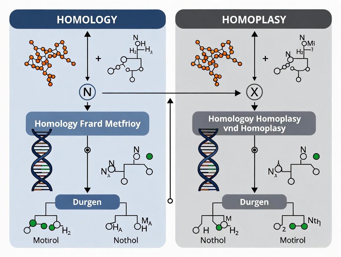
This article provides a comprehensive framework for researchers and drug development professionals to distinguish homology from homoplasy, critical concepts in evolutionary and structural biology.
Homology vs. Homoplasy: A Comprehensive Guide for Biomedical Researchers and Drug Developers
Abstract
This article provides a comprehensive framework for researchers and drug development professionals to distinguish homology from homoplasy, critical concepts in evolutionary and structural biology. We explore the foundational definitions and the continuum between these concepts, detail cutting-edge methodological approaches from phylogenetics to structural bioinformatics, and address common challenges in analysis. A strong emphasis is placed on validation techniques and the direct application of these methods in target identification, lead optimization, and the critical assessment of molecular models in the drug discovery pipeline, empowering scientists to make more accurate evolutionary and functional inferences.
Homology and Homoplasy: Defining the Evolutionary Framework for Biomedical Research
Frequently Asked Questions (FAQs)
1. What is the fundamental difference between homology and homoplasy? Homology describes similarities in sequences or structures due to common evolutionary ancestry. Homoplasy describes similarities that arise independently through convergent evolution, parallel evolution, or evolutionary reversals, not from common ancestry [1] [2].
2. Can a statistically significant BLAST or FASTA result prove homology? Yes. Statistically significant similarity from programs like BLAST, FASTA, or HMMER reliably infers homology, as it indicates "excess similarity" that reflects common ancestry [3].
3. If my sequence search finds no significant matches, does that prove no homologs exist? No. The absence of significant similarity does not prove non-homology. Homologous sequences can diverge to a point where sequence similarity is no longer statistically detectable, leading to false negatives [3].
4. Why is protein sequence alignment more sensitive than DNA alignment for finding distant homologs? Protein alignments have a much longer "evolutionary look-back time" because the genetic code is degenerate, and protein scoring matrices account for conservative amino acid substitutions. Protein-protein alignments can detect homology over billions of years, whereas DNA-DNA alignments rarely detect homology beyond 200-400 million years [3].
5. Are homoplasies just errors in phylogenetic analysis? While sometimes treated as phylogenetic "noise" or errors in preliminary homology assessment, homoplasies are real evolutionary outcomes. Distinguishing between types of homoplasy (e.g., convergence vs. parallelism) can provide valuable insights into evolutionary processes and developmental constraints [2].
Troubleshooting Guides
Problem 1: Interpreting Statistically Significant but Scientifically Unexpected Alignments
Issue: A BLAST search returns a highly significant match (low E-value) to a sequence from a very distant organism, which seems biologically implausible.
Solution:
- Confirm the statistical estimates: Run additional negative control checks.
- Strategy A (Domain Check): Examine the domain content and structural classifications of other high-scoring matches in your results. If sequences with completely different domains also have significant E-values (e.g., < 0.01), the statistical estimates may be unreliable for your query [3].
- Strategy B (Shuffling): Use tools like
SSEARCHfrom the FASTA package to perform statistical estimates based on shuffled versions of your sequence that preserve local amino acid composition. This tests if the high score is a product of sequence composition rather than true homology [3].
- Switch to a more sensitive search: Run a PSI-BLAST or HMMER search to see if the relationship is supported by a profile-based model, which is more robust [3] [4].
Problem 2: Failure to Detect Homologs in a Large Database Search
Issue: A search of a comprehensive database (e.g., NCBI's non-redundant database with >10 million sequences) returns no significant hits.
Solution:
- Search a smaller, specialized database: Try searching a smaller database (<100,000–500,000 entries) that is specific to your organism or protein family of interest. The same alignment score may become statistically significant in a smaller database because the multiple-testing correction is less severe [3].
- Use translated search for DNA queries: If you started with a DNA sequence, use
BLASTXorFASTXto perform a translated search against a protein database. This is far more sensitive for detecting distant evolutionary relationships [3]. - Employ iterative/profile methods: Use tools like
PSI-BLASTorHMMERthat build a profile from initial weak hits to find more distant homologs in subsequent iterations [3] [4].
Problem 3: Distinguishing Homology from Homoplasy in a Phylogenetic Analysis
Issue: A specific character (e.g., a nucleotide, amino acid, or morphological trait) appears to have multiple origins on your phylogenetic tree, suggesting homoplasy.
Solution:
- Calculate the consistency index: Use tools like
HomoplasyFinderto calculate the consistency index for each site in your alignment. This index measures how homoplasious a site is, with lower values indicating greater homoplasy [5]. - Investigate the type of homoplasy: Determine if the homoplasy is convergence, parallelism, or a reversion, as this has evolutionary implications.
- Incorporate EvoDevo data: Investigate whether the genetic or developmental mechanisms underlying the trait are homologous, even if the trait itself appears homoplastic. This can reveal "deep homology" where the generative mechanisms are shared [1] [2].
Key Experimental Protocols
Protocol 1: Conducting a Sensitive Homology Search with BLAST and PSI-BLAST
Objective: To identify both close and distant homologs of a protein sequence.
Materials:
- Query protein sequence in FASTA format.
- Internet connection to access the NCBI BLAST server.
Method:
- Perform a standard protein BLAST (BLASTP):
- Navigate to the NCBI BLAST website.
- Select "protein BLAST" (BLASTP).
- Paste your query sequence and choose the non-redundant protein sequences (nr) database.
- Run the search and note any significant hits (typical E-value threshold < 0.001).
- Perform an iterative PSI-BLAST search:
- On the same BLASTP page, under "Algorithm parameters," change the program from "BLASTP" to "PSI-BLAST."
- Run the initial search.
- PSI-BLAST will return results and allow you to build a PSSM from the significant hits. Use this PSSM to run another iteration.
- Repeat for 3-5 iterations or until no new significant domains are found. Convergence indicates a robust profile has been built [4].
Troubleshooting: If PSI-BLAST incorporates unrelated sequences (a "runaway" search), manually inspect and exclude questionable sequences from the PSSM building step before the next iteration.
Protocol 2: Identifying Homoplasious Sites in a Phylogenetic Alignment
Objective: To find sites in a DNA or protein sequence alignment that are inconsistent with a given phylogenetic tree.
Materials:
- A multiple sequence alignment (FASTA, PHYLIP, or NEXUS format).
- A corresponding phylogenetic tree (Newick format) for the sequences in the alignment.
- The
HomoplasyFinderR package [5].
Method:
- Install HomoplasyFinder: In your R environment, install and load the package.
- Run the analysis: Provide the alignment and tree files to the
homoplasyFinderfunction. The tool will calculate the consistency index for each site in the alignment. - Interpret the output: The output will identify sites with a consistency index less than 1. These are homoplasious sites. A site with a perfect consistency index of 1 is fully consistent with the tree (non-homoplasious) [5].
Data Presentation
Table 1: Statistical Thresholds for Inferring Homology from Sequence Searches
| Search Type | Program Examples | Recommended E-value Threshold | Key Considerations |
|---|---|---|---|
| Protein-Protein | BLASTP, FASTA, SSEARCH | < 0.001 [3] | Reliable for inferring homology and structural similarity. |
| Translated DNA-Protein | BLASTX, FASTX | < 0.001 [3] | Much more sensitive than DNA-DNA searches for distant homologs. |
| DNA-DNA | BLASTN, MEGABLAST | < 10^-10 [3] | DNA alignment statistics are less accurate; a much stricter threshold is required. |
Table 2: Comparison of Homoplasy Types and Their Significance
| Type | Definition | Underlying Cause | Evolutionary Significance |
|---|---|---|---|
| Convergence | Independent evolution of similar traits in unrelated lineages. | Different developmental/genetic generators (non-homologous) [2]. | Demonstrates power of natural selection to produce similar adaptations from different starting points [2]. |
| Parallelism | Independent evolution of similar traits in closely related lineages. | Similar developmental/genetic generators (homologous) from a common ancestor [2]. | Suggests shared developmental constraints; can be considered a class of homology [1] [2]. |
| Reversion | A trait reverts from a derived state back to a state resembling its ancestral form. | Can involve reactivation of ancestral genetic pathways. | Indicates underlying genetic potential for a trait can be retained over evolutionary time [1]. |
Workflow and Relationship Visualizations
| Tool / Resource | Function | Example Use Case |
|---|---|---|
| BLAST Suite | Finds regions of local similarity between sequences; infers homology [3]. | Initial characterization of a newly sequenced gene. |
| PSI-BLAST | Builds a PSSM from BLAST results for more sensitive, iterative searches [4]. | Detecting very distant homologs missed by standard BLAST. |
| HMMER | Uses hidden Markov models for sensitive sequence similarity searches and family profiling. | Identifying members of a protein domain family in a genome. |
| Multiple Alignment Tools (e.g., MUSCLE, MAFFT) | Aligns three or more sequences to identify conserved regions [6]. | Preparing data for phylogenetic tree building. |
| HomoplasyFinder | Identifies homoplasious sites in an alignment given a phylogeny using the consistency index [5]. | Pinpointing sites under potential selection or involved in convergent evolution. |
| Phylogenetic Software (e.g., MrBayes, RAxML) | Infers evolutionary relationships (phylogenetic trees) from sequence data. | Testing hypotheses of common descent and mapping character evolution. |
| PDB (Protein Data Bank) | Repository for experimentally determined 3D structures of proteins and nucleic acids [4]. | Template for homology modeling; verifying structural homology. |
| SWISS-MODEL, Phyre2 | Automated servers for protein structure homology modeling [4]. | Predicting the 3D structure of a protein when no experimental structure exists. |
Theoretical Framework: Understanding the Continuum
Fundamental Definitions and the Spectrum Concept
The classical biological distinction between homology and homoplasy represents not a strict dichotomy but rather a continuum of evolutionary relationships. Homology is defined as the presence of the same feature in two organisms whose most recent common ancestor also possessed that feature, reflecting similarity due to common descent and ancestry [7] [1]. In contrast, homoplasy refers to similarity arrived at through independent evolution, including convergence, parallelism, and evolutionary reversal [7] [8]. The continuum perspective recognizes that all organisms share some degree of relationship through the single tree of life, with features exhibiting varying degrees of ancestral connection versus independent origin [1].
This framework reveals a spectrum extending from homology → reversals → rudiments → vestiges → atavisms → parallelism, with convergence as the primary category of true homoplasy [1] [9]. This realignment helps bridge phylogenetic and developmental approaches to evolutionary biology, directing researchers toward searching for common elements underlying phenotype formation rather than focusing exclusively on shared versus independent evolution [1].
Categories of Homoplasy and Their Developmental Bases
Table: Categories of Homoplasy and Their Characteristics
| Category | Developmental Basis | Evolutionary Mechanism | Research Implications |
|---|---|---|---|
| Convergence | Different developmental pathways | Independent evolution under similar selective pressures | Search for different genetic mechanisms producing similar forms |
| Parallelism | Similar or identical developmental mechanisms | Independent evolution reusing conserved developmental programs | Identify deeply conserved genetic pathways recruited independently |
| Reversals/Atavisms | Retention of ancestral developmental potential | Reactivation of suppressed ancestral genetic programs | Investigate gene regulatory network stability and suppression mechanisms |
| Rudiments/Vestiges | Conservation of developmental pathways despite structural reduction | Loss of selective maintenance while developmental capacity persists | Study gene expression patterns in reduced structures |
Research indicates these categories have distinct developmental bases: convergence arises through different developmental pathways, parallelism utilizes similar developmental mechanisms, while reversals and atavisms employ similar or divergent developmental mechanisms to reactivate ancestral traits [7]. Structures may be lost evolutionarily while their developmental foundations remain, creating potential for homoplasy when these latent programs are reactivated [7].
Methodological Approaches: Technical Protocols
Homology Modeling in Drug Discovery: A Stepwise Protocol
Homology modeling enables prediction of 3D protein structures when experimental structures are unavailable, with significant applications in drug discovery [10] [11]. The quality of resulting models directly correlates with sequence identity between target and template.
Table: Homology Modeling Quality Versus Sequence Identity
| Sequence Identity | Model Quality & Applications | Limitations & Considerations |
|---|---|---|
| >50% | Sufficient for drug discovery applications; reliable prediction of protein-ligand interactions | High confidence in backbone and side chain positioning |
| 30-50% | Useful for predicting target druggability, designing mutagenesis experiments, and in vitro test design | Moderate confidence; requires careful validation |
| 15-30% | Fold assignment possible with sophisticated methods; limited to functional assignment | Conventional alignment methods unreliable; requires profile-based methods |
| <15% | Modeling becomes speculative; high risk of misleading conclusions | Threading methods may be applied but with limited confidence |
Experimental Protocol: Homology Modeling Workflow
Step 1: Template Identification and Fold Recognition
- Input target amino acid sequence into BLAST (https://www.ncbi.nlm.nih.gov/BLAST/) against Protein Data Bank (PDB) database
- For distant homologs (<30% identity), use iterative PSI-BLAST or Hidden Markov Models (HMMER, SAM-T98)
- Validate potential templates using structural classification databases (SCOP, CATH)
- Troubleshooting Tip: If BLAST fails to identify templates, use profile-profile alignment methods (FFAS03, HHsearch) or threading approaches
Step 2: Multiple Sequence Alignment
- Align target sequence with identified templates using ClustalW, ClustalX, or T-Coffee
- For improved accuracy with divergent sequences, use PROBCONS or incorporate structural information with 3D-Coffee
- Manually inspect alignment for conserved functional motifs and structural domains
- Troubleshooting Tip: Use HOMSTRAD or BAliBASE reference alignments to validate alignment approach
Step 3: Model Building
- Generate initial model using MODELLER, SWISS-MODEL, or alternative modeling software
- Apply rigid-body assembly for conserved core regions
- Model loops using segment matching or conformational search restrained by energy functions
- Troubleshooting Tip: Generate multiple models to account for alignment ambiguities
Step 4: Model Refinement and Validation
- Energy minimization using molecular mechanics force fields (AMBER, CHARMM)
- Molecular dynamics simulation for conformational sampling
- Validate model geometry using PROCHECK, Verify3D, or MolProbity
- Troubleshooting Tip: Assess model quality by determining if >90% of residues fall in favored regions of Ramachandran plot
Distinguishing Homology from Homoplasy: Phylogenetic Protocol
Experimental Protocol: Phylogenetic Discrimination Method
Step 1: Character State Identification
- Clearly define the trait or feature being compared across taxa
- Specify the level of biological organization (gene, protein, structure, behavior)
- Document character states for each taxon in the analysis
- Troubleshooting Tip: Ensure homologous comparisons specify both the organisms being compared and the specific aspect of the trait being examined [8]
Step 2: Phylogenetic Tree Construction
- Select appropriate molecular markers (conserved genes for deep relationships, rapidly evolving markers for recent divergences)
- Apply multiple phylogenetic methods (maximum parsimony, maximum likelihood, Bayesian inference)
- Assess node support with bootstrapping or posterior probabilities
- Troubleshooting Tip: Compare trees generated from different marker sets to identify potential incongruences
Step 3: Character Mapping and Optimization
- Map character states onto the phylogenetic tree
- Reconstruct ancestral states using parsimony or likelihood methods
- Identify synapomorphies (shared derived traits) indicating homology
- Troubleshooting Tip: Use multiple reconstruction methods to assess sensitivity of ancestral state inferences
Step 4: Testing for Homoplasy
- Calculate consistency index and retention index to quantify homoplasy
- Use statistical tests (Shimodaira-Hasegawa test, SOWH test) to compare constrained and unconstrained trees
- Apply specific methods to detect convergent evolution (CONVERGE software)
- Troubleshooting Tip: High homoplasy levels may indicate conserved genetic/developmental mechanisms underlying character evolution [7]
Frequently Asked Questions: Technical Troubleshooting
Conceptual and Theoretical Questions
Q1: How can we distinguish between homologous and homoplasious traits when they look remarkably similar? A1: The distinction requires multiple lines of evidence beyond superficial similarity:
- Phylogenetic distribution: Homologous traits follow expected patterns of common descent, while homoplasious traits appear in distantly related lineages
- Developmental pathways: Homologous traits typically share deeper developmental mechanisms, even when modified
- Genetic basis: Homologous traits often involve orthologous genes, while homoplasy may involve different genetic mechanisms or parallel changes in the same genes
- Fossil evidence: When available, fossil sequences can reveal historical transitions
Q2: Can a trait be homologous at one biological level but homoplasious at another? A2: Yes, this hierarchical perspective is crucial for accurate analysis. For example:
- Vertebrates and cephalopods have homoplasious complex eyes as organs, but share homologous cell types and the Pax6 control gene [8]
- Zeta-crystallin is homologous as a molecule in llamas and guinea pigs but homoplasious as a lens component, as it was independently recruited for this function [8]
- Always specify both the organisms being compared and the specific aspect of the trait under investigation
Q3: What is "deep homology" and how does it relate to the continuum concept? A3: Deep homology refers to shared genetic and developmental mechanisms underlying traits in distantly related organisms, even when the structures themselves are not homologous. This concept supports the continuum view by demonstrating that:
- Similar features can persist when present in a common ancestor (traditional homology)
- Different environments can trigger reappearance of similar features using conserved genetic toolkits (homoplasy with deep homology)
- Structures may be evolutionarily lost while developmental potential persists [7]
Technical and Methodological Questions
Q4: What sequence identity threshold is needed for reliable homology modeling in drug discovery? A4: Sequence identity requirements depend on the application:
- >50% identity: Models sufficient for drug discovery applications and predicting protein-ligand interactions
- 30-50% identity: Useful for predicting target druggability and designing mutagenesis experiments
- 15-30% identity: Limited to fold assignment and guiding experimental approaches
- <15% identity: Models are speculative and may lead to incorrect conclusions [10] [11]
Q5: How can we minimize alignment errors in homology modeling, especially with low sequence identity? A5: Address alignment errors through these approaches:
- Use iterative search methods (PSI-BLAST) rather than simple pairwise alignment
- Apply profile-based methods (Hidden Markov Models) for distant homologs
- Incorporate structural information when available (3D-Coffee)
- Generate and compare multiple alignments using different methods
- Manually inspect alignments in regions of functional importance (active sites, binding pockets)
Q6: What validation methods are essential for assessing homology model quality? A6: Essential validation includes:
- Geometric checks: Ramachandran plots, side-chain rotamer distributions, and steric clashes
- Energetic assessment: Calculation of residue knowledge-based potentials
- Comparison with experimental data: Mutagenesis results, biochemical data
- Evolutionary conservation: Analysis of conserved vs. variable regions
- Critical step: Always validate models before use in drug design projects
Research Reagent Solutions: Essential Materials
Table: Key Research Reagents and Databases for Homology/Homoplasy Research
| Reagent/Database | Function/Purpose | Access Information | Application Notes |
|---|---|---|---|
| Protein Data Bank (PDB) | Repository of experimentally determined protein structures | http://www.rcsb.org/pdb | Foundation for template identification in homology modeling |
| SWISS-MODEL Repository | Database of annotated comparative protein structure models | http://swissmodel.expasy.org/repository | Provides pre-computed models for many protein sequences |
| ModBase | Database of comparative protein structure models | http://modbase.compbio.ucsf.edu | Contains models for ~56% of known protein sequences |
| BLAST Suite | Sequence similarity search and alignment tools | http://www.ncbi.nlm.nih.gov/BLAST | Initial template identification and sequence comparison |
| ClustalW/ClustalX | Multiple sequence alignment programs | Various implementations | Standard tools for creating target-template alignments |
| MODELLER | Homology modeling software | Academic license available | Widely used for comparative model building |
| HMMER | Hidden Markov Model implementation for sequence analysis | http://hmmer.org | Sensitive detection of distant homologs |
| Pax6 Antibodies | Detection of conserved transcription factor in eye development | Commercial suppliers | Experimental validation of deep homology relationships |
| BAliBASE | Reference alignment database for method validation | http://www.lbgi.fr/balibase | Benchmarking alignment accuracy |
Advanced Visualization: Conceptual Relationships
FAQ: Core Concepts and Definitions
What is the fundamental difference between homology and homoplasy? Homology is a relation of correspondence between parts of organisms that derive from a common ancestral precursor. Homology is a transitive relation, meaning homologues remain homologous however much they may differ over evolutionary time. In contrast, homoplasy is an umbrella term encompassing convergent, parallel, and reversal evolution, where similar features arise independently not from common ancestry but due to similar evolutionary pressures or constraints [12].
How does convergence differ from parallelism? Convergence and parallelism are both forms of homoplasy but have a crucial distinction based on ancestral traits and underlying mechanisms. Convergence occurs when two species independently evolve similar traits from dissimilar ancestral states and often involve non-homologous underlying genetic or developmental generators. Parallelism occurs when two species independently evolve similar traits from a similar ancestral state, often utilizing homologous developmental pathways or genetic machinery [2] [13]. Parallelism can be considered a "gray zone" between homology and convergence because it involves common ancestry at the level of the developmental generators [2].
What are evolutionary reversals, and how are they classified? An evolutionary reversion, or reversal, occurs when a lineage returns to an ancestral, plesiomorphic state from a derived, apomorphic state. In cladistic literature, reversions are often interpreted as a form of convergence [2]. They represent a specific type of homoplasy where a trait is lost and then reappears in a later descendant.
Why is it important for phylogeneticists to distinguish between these types of homoplasy? While some cladistic methods treat all homoplasy as an "error" or phylogenetic noise, distinguishing its type provides valuable evolutionary insights. Recognizing parallelism can provide evidence of common ancestry through shared developmental constraints, whereas convergence highlights the power of natural selection in shaping analogous adaptations in different lineages. Incorporating evidence from EvoDevo helps test different evolutionary hypotheses beyond the phylogenetic tree topology itself [2].
FAQ: Troubleshooting Phylogenetic Analysis
My phylogenetic analysis shows a trait with a discontinuous distribution. How can I determine if it is homology or homoplasy? The initial test is character congruence within a cladistic framework. Characters that are congruent and support the same clade are considered homologous (synapomorphies), while incongruent characters that conflict with the clade are initially considered homoplastic [2]. However, this should be followed by investigating the underlying biology:
- Actionable Protocol: Investigate the genetic and developmental basis of the trait. If the same homologous genes and developmental pathways are responsible for the trait in the different lineages, it is evidence for parallelism. If different genetic mechanisms produce the phenotypically similar trait, it is evidence for convergence [2].
I have identified a homoplasy. What experimental approaches can distinguish convergence from parallelism? The key is to move beyond the pattern of trait distribution and investigate the mechanistic processes.
- Actionable Protocol:
- EvoDevo Analysis: Compare the developmental pathways that generate the trait in the different lineages. This involves gene expression studies (e.g., in situ hybridization) and functional tests (e.g., CRISPR knockouts).
- Genetic Analysis: Identify the genes and mutations responsible for the trait. Orthologous genes with similar mutations suggest parallelism, while different genes or non-homologous mutations suggest convergence.
- Assess Ancestral State: Reconstruct the ancestral condition for both the trait and the underlying genetic/developmental system. Similar ancestral states for both indicate potential for parallelism [2] [13].
How can I visualize sequence data to identify conserved and variable regions that might indicate homoplasy? Multiple sequence alignments (MSAs) are fundamental. While traditional "stacked sequence" visualizations can be inadequate for large datasets, newer paradigms like Sequence Logos and ProfileGrids are effective.
- Actionable Protocol: Use tools like JProfileGrid or WebLogo to visualize your MSAs [14]. ProfileGrids represent an alignment as a color-coded matrix of residue frequency, providing a clear "heat map" of conservation and diversity. This allows for easy identification of positions that are highly conserved (potential homology) or highly variable (potential sites for homoplasy). Unlike Sequence Logos, ProfileGrids keep all residue symbols legible, which is critical for interpreting variable columns [14].
My sequence alignment is large and complex. What visualization tools can help me analyze it effectively? The "row-column" paradigm for MSAs becomes insufficient with large datasets. The ProfileGrid paradigm, implemented in the JProfileGrid software, is designed for this purpose.
- Actionable Protocol: Input your alignment into JProfileGrid. It reduces the alignment to a matrix color-shaded according to residue frequency, allowing you to see overall conservation trends. A key feature is interactivity; you can select any cell in the ProfileGrid to query the underlying MSA data, enabling you to identify sequences with rare residues and investigate potential homoplasies in detail [14].
Data Tables
Table 1: Diagnostic Characteristics of Homology and Homoplasy
| Category | Definition | Ancestral State | Underlying Mechanism | Evolutionary Implication |
|---|---|---|---|---|
| Homology | Correspondence due to common ancestry [12] | Same common ancestor | Shared genetic/developmental basis (homologous generators) | Evidence of common descent |
| Convergence | Independent evolution of similar features from dissimilar ancestors [13] | Dissimilar | Different genetic/developmental basis (non-homologous generators) [2] | Evidence of adaptation and natural selection |
| Parallelism | Independent evolution of similar features from similar ancestors [13] | Similar | Shared genetic/developmental basis (homologous generators) [2] | Evidence of developmental constraint and common ancestry of generators |
| Reversal | Return to an ancestral character state [2] | Previously existed | Can involve reactivation of ancestral genetic pathways | Can obscure phylogenetic relationships |
Table 2: Molecular and Phenotypic Examples of Homoplasy
| Category | Classic Phenotypic Example | Molecular Example |
|---|---|---|
| Convergence | Camera eyes in cephalopods and vertebrates [13] | Protease catalytic triads evolving independently over 20 times in different enzyme superfamilies [13] |
| Parallelism | Gliding frogs evolving independently from multiple types of tree frog [13] | Parallel amino acid substitutions in the Na+,K+-ATPase enzyme for cardiotonic steroid resistance in insects [13] |
| Reversal | Re-evolution of lost traits (atavisms) | Re-activation of silenced genes or developmental pathways to produce an ancestral phenotype [13] |
Experimental Protocols and Workflows
Protocol 1: A Workflow for Diagnosing Homoplasy
This protocol outlines a step-by-step methodology for investigating a suspected case of homoplasy, from initial phylogenetic observation to mechanistic confirmation.
Protocol 2: Generating a ProfileGrid for MSA Visualization
This protocol details the steps to create and interpret a ProfileGrid visualization for analyzing conservation and variation in large multiple sequence alignments, a key step in identifying potential homoplastic sites.
The Scientist's Toolkit: Research Reagent Solutions
Table 3: Essential Resources for Homoplasy Research
| Tool / Reagent | Function / Purpose | Example / Specification |
|---|---|---|
| Multiple Sequence Alignment Software | Aligns homologous sequences from different taxa to identify corresponding positions. | Software like ClustalOmega, MAFFT, or MUSCLE [14]. |
| Phylogenetic Analysis Package | Reconstructs evolutionary relationships and tests character evolution. | Packages like PAUP*, MrBayes, or BEAST. |
| Substitution Matrix (e.g., BLOSUM, PAM) | Quantifies the likelihood of amino acid substitutions; basis for alignment scores and can inform color schemes in visualization [15]. | BLOSUM62 is a standard matrix for protein alignment. |
| Visualization Tools (ProfileGrid/Sequence Logo) | Creates intuitive visual summaries of sequence conservation and variation in alignments [14]. | JProfileGrid.org (for ProfileGrids) or WebLogo (for Sequence Logos) [14]. |
| Genome Databases | Provides raw sequence data for phylogenetic and comparative analysis. | NCBI GenBank, Ensembl, UniProt. |
| Developmental Biology Reagents | For investigating mechanisms (parallelism vs. convergence). Includes tools for gene expression and functional analysis. | Antibodies for specific proteins, in situ hybridization kits, CRISPR-Cas9 tools for functional tests. |
The Critical Role of Common Ancestry in Functional Inference for Drug Targets
In the pursuit of effective therapeutic targets for complex diseases, distinguishing between homology (similarity due to common ancestry) and homoplasy (similarity arising independently) is a fundamental challenge in evolutionary biology with direct implications for drug discovery. Homoplasy, often perceived negatively in cladistic analysis as "error in our preliminary assignment of homology" [2], encompasses convergence, parallelism, and reversions. However, from an evolutionary perspective, homoplasy—particularly parallelism—can provide crucial insights when it results from similar developmental constraints in related lineages [2]. Genomic evidence now demonstrates that therapeutic targets with genetic support are twice as likely to succeed in clinical trials [16], making accurate evolutionary inference essential for distinguishing genuinely conserved biological pathways from superficially similar traits. This technical support center provides methodologies for resolving these evolutionary relationships to enhance target validation in drug development.
Troubleshooting Guides & FAQs
FAQ: Evolutionary Concepts in Target Validation
Q1: How does distinguishing homology from homoplasy improve drug target validation?
Accurate distinction prevents misallocation of resources by identifying targets with genuine evolutionary conservation versus those with superficial functional similarities. Homologous targets share conserved biological pathways due to common ancestry, offering higher translational potential across species in preclinical studies. In contrast, homoplastic similarities may represent convergent functions through different mechanisms, increasing the risk of failure in later stages. Research indicates that drugs with genetically supported targets are twice as likely to progress through clinical trial phases [16], underscoring the importance of evolutionary validation.
Q2: What analytical frameworks integrate evolutionary principles with genomic data for target identification?
Summary-data-based Mendelian Randomization (SMR) provides a robust framework linking genetic variants to disease risk through molecular intermediates like gene expression (eQTLs), protein abundance (pQTLs), and chromatin accessibility (caQTLs) [16]. This approach tests whether pleiotropic association between exposure (QTL) and outcome (disease) stems from shared causal variants or mediation, effectively distinguishing conserved biological pathways from spurious associations. The accompanying HEIDI (heterogeneity in dependent instruments) method further discriminates whether associations arise from pleiotropy (potentially homologous) versus linkage (potentially homoplastic) [16].
Q3: How can researchers determine if similar traits in model organisms and humans represent homology or homoplasy?
Comparative genomic analysis across multiple species establishes whether shared traits derive from common ancestry. Key criteria include:
- Shared genetic basis: Orthologous genes and conserved regulatory elements indicate homology
- Developmental constraints: Similar underlying generative mechanisms suggest parallelism
- Phylogenetic distribution: Traits following established evolutionary relationships support homology True parallelism involves phenotypic recurrence due to homologous underlying generators (developmental or genetic), while convergence utilizes non-homologous generators despite similar functions [2].
Troubleshooting Guide: Common Experimental Challenges
Problem: Spurious correlation between gene expression and disease risk
Solution: Implement SMR with HEIDI testing to distinguish causal relationships from linkage.
- Obtain summarized eQTL and GWAS data from relevant tissues
- Apply SMR to test pleiotropic association between expression and disease
- Use HEIDI test (p > 0.01 indicates pleiotropy) to exclude linkage
- Validate through colocalization analysis assessing shared causal variants [16]
Problem: Uncertain translational relevance of targets identified in model systems
Solution: Establish evolutionary relationships through cross-species analysis.
- Perform phylogenetic analysis of target gene across species of interest
- Identify conserved functional domains and regulatory elements
- Assess expression patterns in homologous cell types/tissues
- Validate functional conservation through experimental perturbation in multiple systems [16] [17]
Problem: Ancestral confounding in target-disease associations
Solution: Apply Mendelian Randomization with post-selection inference (MR-SPI).
- Select genetic instruments from pQTL data (P < 1.70×10⁻¹¹)
- Implement MR-SPI voting procedure to distinguish valid from invalid instruments
- Estimate causal effect of protein on disease risk
- Validate through sensitivity analyses and colocalization [17]
Data Presentation: Quantitative Evidence
Table 1: Neurodegenerative Disease Target Genes Identified Through SMR Framework
| Disease | Number of Identified Target Genes | Novel Targets | Known Targets | Difficult Targets |
|---|---|---|---|---|
| Alzheimer's Disease | 116 | 41 | 3 | 115 |
| Amyotrophic Lateral Sclerosis | 3 | - | - | - |
| Lewy Body Dementia | 5 | - | - | - |
| Parkinson's Disease | 46 | - | - | - |
| Progressive Supranuclear Palsy | 9 | - | - | - |
Data sourced from omicSynth resource identifying therapeutic targets for neurodegenerative diseases through SMR analysis (pSMR_multi < 2.95 × 10⁻⁶ and pHEIDI > 0.01) [16].
Table 2: Atrial Fibrillation Genetic Discovery Metrics
| Analysis Type | Number of Genome-Wide Significant Variants | Novel Variants | Genes Identified | Proteins Associated |
|---|---|---|---|---|
| GWAS Meta-analysis | 244 | 77 | - | - |
| Transcriptome-Wide Association Study | - | - | 372 | - |
| Proteome-Wide MR Analysis | - | - | - | 155 |
Results from genomic data-driven framework for AF drug target discovery, integrating GWAS meta-analysis of 1,347,178 participants with transcriptomic and proteomic data [17].
Experimental Protocols
Purpose: Test causal relationships between molecular traits (e.g., gene expression) and complex diseases using summarized genetic data.
Materials:
- GWAS summary statistics for disease of interest
- QTL data (eQTL, pQTL, mQTL, or caQTL) from relevant tissues
- SMR software (available from Yang Lab)
- LD reference panel matching QTL data
Methodology:
- Data Preparation: Process GWAS and QTL data to consistent genome build (e.g., hg19). Apply quality controls: MAF > 0.1%, imputation quality scores > 0.6.
- SMR Analysis: Test pleiotropic association between molecular trait (exposure) and disease (outcome) using the SMR statistic, which follows a chi-square distribution with one degree of freedom.
- HEIDI Test: Distinguish pleiotropy from linkage using multiple cis-QTLs. Retain associations with HEIDI p-value > 0.01.
- Multiple Testing Correction: Apply stringent threshold (pSMR_multi < 2.95 × 10⁻⁶) to account for genome-wide testing [16].
- Biological Validation: Assess target expression in disease-relevant cell types using single-nucleus RNA sequencing data.
Protocol 2: Genetic Colocalization Analysis
Purpose: Determine whether two traits share the same causal genetic variant in a genomic region.
Materials:
- GWAS summary statistics for disease and molecular trait
- Colocalization software (e.g., COLOC)
- LD matrix from reference panel
Methodology:
- Define Regions: Identify genomic regions containing significant associations for both traits.
- Bayesian Testing: Compute posterior probabilities for five colocalization hypotheses using default prior probabilities.
- Threshold Application: Classify strong colocalization evidence when posterior probability > 0.80 for shared causal variant hypothesis.
- Sensitivity Analysis: Test robustness to prior specification and LD estimation [17].
Research Workflow Visualization
Evolutionary Genomics Target Identification Workflow
Research Reagent Solutions
| Resource | Function | Application in Target Discovery |
|---|---|---|
| GWAS Summary Statistics | Provides genetic associations with complex diseases | Identify potential target-disease relationships through variant associations [16] [17] |
| QTL Data (eQTL/pQTL/mQTL/caQTL) | Maps genetic variants to molecular phenotypes | Establish functional links between variants and gene/protein expression [16] |
| LD Reference Panels | Characterizes correlation structure between variants | Account for population structure in genetic analyses [16] [17] |
| Single-Nucleus RNA Sequencing Data | Profiles gene expression at cellular resolution | Verify target expression in disease-relevant cell types [16] |
| SMR/HEIDI Software | Implements Mendelian randomization framework | Test causal relationships and distinguish homology from homoplasy [16] |
| Colocalization Tools (COLOC) | Bayesian test for shared causal variants | Confirm shared genetic mechanisms between traits [17] |
Integrating evolutionary principles with genomic data provides a powerful framework for distinguishing biologically conserved therapeutic targets from spurious associations. The methodologies outlined in this technical support center enable researchers to leverage common ancestry as evidence for functional conservation while accounting for evolutionary independent similarities that may mislead target selection. As drug discovery increasingly relies on genetic evidence, these approaches will be essential for prioritizing targets with the highest probability of clinical success.
Troubleshooting Guide: Common Issues in Homology vs. Homoplasy Research
FAQ: How do I distinguish a true homology from a homoplasy in my gene sequence data? True homology, or "the same organ in different animals under every variety of form and function" [18], implies shared ancestry. Homoplasy (analogy) describes structures with the same function but different evolutionary origins [18]. To distinguish them in your data:
- Method: Conduct phylogenetic analysis and sequence alignment.
- Expected Result: For homologous genes, sequence similarity is high in closely related species and the gene tree should match the species tree.
- Troubleshooting: If you find similar sequences in distantly related species, but the similarity is confined to a short, functional domain, and the gene tree is inconsistent with the species tree, this suggests homoplasy due to convergent evolution.
FAQ: My gene expression patterns are inconsistent across species. Does this rule out homology? Not necessarily. Homology is about evolutionary origin, not identical developmental pathways [18] [19].
- Method: Compare the gene's regulatory network and its positional relationships within the genome (synteny), not just its expression pattern.
- Expected Result: A deeply conserved regulatory gene or network might be expressed in different tissues in different species but still be homologous.
- Troubleshooting: Investigate if the gene is part of a conserved gene regulatory network (GRN). Homologous genes often have conserved upstream regulators or target genes, even if their precise expression domain has shifted.
FAQ: What is the best way to analyze biomineralization proteins across different taxa? Biomineralization proteins are a key model for studying the evolution of complex traits [20].
- Method: Use comparative genomics and transcriptomics. Sequence the transcriptomes of biomineralizing tissues (e.g., the mantle in mollusks) and curate proteins into a specialized database like BioMine-DB [20].
- Expected Result: You will identify shared protein families and lineage-specific innovations.
- Troubleshooting: If a protein family appears absent, check for high sequence divergence. Use sensitive profile-based search methods (e.g., HMMER) to detect distant homologs.
Experimental Protocols for Key Evo-Devo Experiments
Protocol 1: Transcriptome Sequencing for Biomineralization Gene Discovery This protocol is based on methods used to increase phylogenetic representation of lophotrochozoan biomineralization genetics [20].
- Tissue Collection: Dissect biomineralizing tissue (e.g., mollusk mantle) and preserve immediately in RNAlater.
- RNA Extraction: Use a standard phenol-chloroform extraction or commercial kit to obtain high-quality, intact RNA.
- Library Preparation & Sequencing: Construct cDNA libraries and sequence using an Illumina platform to generate high-coverage, paired-end reads.
- Transcriptome Assembly & Annotation: De novo assemble reads into transcripts using a tool like Trinity. Annotate transcripts by comparing them to public databases (e.g., UniProt, Pfam) using BLAST.
- Identification of Biomineralization Proteins: Curate a list of known biomineralization proteins and identify homologs within your annotated transcriptome.
Protocol 2: Testing for Homology using Phylogenetic and Synteny Analysis
- Sequence Identification: Identify your gene of interest in the target species using BLAST.
- Multiple Sequence Alignment: Gather homologous sequences from a wide range of taxa and perform a multiple sequence alignment with a tool like MUSCLE or MAFFT.
- Phylogenetic Tree Construction: Build a gene tree using maximum likelihood (e.g., RAxML) or Bayesian (e.g., MrBayes) methods.
- Synteny Analysis: Examine the genomic region surrounding your gene in multiple species to see if the same neighboring genes are conserved.
- Interpretation: A gene that groups with strong statistical support on the species tree and resides in a region of conserved synteny is likely a true homology. A gene that appears in distantly related taxa without synteny support may be a homoplasy.
Table 1: Key Historical Concepts and Definitions in Evolutionary Morphology
| Concept | Proponent(s) | Definition | Significance for Evo-Devo |
|---|---|---|---|
| Homology | Richard Owen (1843) [18] | "The same organ in different animals under every variety of form and function." | Establishes the basis for comparing anatomical structures across species based on common ancestry. |
| Analogy | Richard Owen (1843) [18] | "A part or organ in one animal which has the same function as another part or organ in a different animal." | Now called homoplasy; critical for identifying convergent evolution. |
| Unity of Type | (Pre-Darwin) | Similarity in the general plan of organisation within a class of organisms [21]. | Provided evidence for common descent; explained by deep homology in developmental genes. |
| Archetype | Richard Owen [21] | A predetermined, ideal pattern or "idea" underlying the structure of a group of organisms. | A pre-evolutionary concept that contrasted with Darwin's common descent explanation for unity of type. |
Table 2: Essential Research Reagent Solutions for Evo-Devo Studies
| Reagent / Material | Function / Application |
|---|---|
| RNAlater | Stabilizes and protects RNA in tissues collected for transcriptome sequencing [20]. |
| BioMine-DB | A biomineralization-centric protein database for curating and comparing relevant proteins [20]. |
| Phusion High-Fidelity DNA Polymerase | For accurate PCR amplification of genes for phylogenetic analysis or cloning. |
| Whole Genome/Transcriptome Data | Essential for comparative genomics, synteny analysis, and identifying homologous genes [20] [18]. |
Logical Workflow and Signaling Pathway Diagrams
Diagram 1: Decision workflow for distinguishing homology from homoplasy.
Diagram 2: Central dogma and the genotype-phenotype map in evolution.
Methodologies in Action: From Phylogenetics to Homology Modeling in Drug Discovery
In phylogenetic systematics, the principle of character congruence is the fundamental method used to test hypotheses of homology. Homology is the presence of the same feature in two organisms whose most recent common ancestor also possessed that feature [22]. Character congruence involves comparing multiple character distributions across taxa to distinguish true homologies (synapomorphies) from homoplasies (similar traits not derived from a common ancestor) [2]. This methodological approach stands in contrast to the traditional concept of the homology/homoplasy dichotomy, with many contemporary researchers now viewing these concepts as existing along a continuum rather than as absolute categories [22].
The process of distinguishing homology from homoplasy is critical for reconstructing accurate evolutionary relationships. Homoplasy represents independent evolution of similar characteristics and can manifest as convergence, parallelism, or reversals [2]. While traditionally viewed as "phylogenetic noise" that obscures evolutionary relationships, contemporary evolutionary biology recognizes that detailed investigation of homoplasy can provide valuable insights into evolutionary processes, particularly when integrated with evidence from evolutionary developmental biology (EvoDevo) [2]. This technical guide addresses common challenges researchers face when applying character congruence methods in their phylogenetic analyses.
Frequently Asked Questions (FAQs)
What is the practical difference between homology and homoplasy in phylogenetic analysis? Homology describes traits shared due to common ancestry that provide evidence for evolutionary relationships. Homoplasy describes similar traits that arise independently in different lineages due to convergent evolution, parallel evolution, or evolutionary reversals. In practice, homology is determined through character congruence tests during phylogenetic analysis - characters that are congruent (group the same taxa) are considered homologous, while incongruent characters are considered homoplastic [2].
How can I distinguish between parallelism and convergence in my character data? Parallelism involves independent evolution of similar traits through the same underlying developmental or genetic mechanisms inherited from a common ancestor, while convergence involves similar traits arising through different developmental mechanisms [2]. Distinguishing between them requires integrating evidence from evolutionary developmental biology (EvoDevo) to examine whether the same genetic pathways generate the similar traits in different lineages [2].
Why does my phylogenetic analysis show conflicting signals between different character sets? Conflicting signals often result from homoplasy in one or more character sets, but may also stem from methodological issues including inadequate taxon sampling, long-branch attraction, or different evolutionary rates among lineages [23] [2]. Poor taxon sampling may result in incorrect phylogenetic inferences, and long branch attraction can cause unrelated branches to be incorrectly grouped by shared, homoplastic characters [23].
What does it mean when my morphological and molecular data support different tree topologies? Incongruence between morphological and molecular datasets may indicate homoplasy in one dataset, but may also reflect differences in evolutionary rates, incomplete lineage sorting, or the action of different selective pressures on morphological versus molecular characters. Such conflicts require careful investigation of potential homoplasy in both datasets rather than assuming one dataset is inherently more reliable [2].
Troubleshooting Common Experimental Problems
Homoplasy Identification and Resolution
Table 1: Troubleshooting Homoplasy Detection in Phylogenetic Analysis
| Problem | Potential Causes | Solutions |
|---|---|---|
| High homoplasy levels in character matrix | Character coding issues; true evolutionary convergence; inadequate taxon sampling | Review character state definitions; add taxa to break long branches; consider alternative evolutionary models |
| Incongruence between data partitions | Different evolutionary histories; homoplasy in one partition; different evolutionary rates | Conduct partition homogeneity tests; analyze partitions separately; integrate EvoDevo evidence to test homology hypotheses [2] |
| Poor nodal support despite low homoplasy | Insufficient phylogenetic signal; conflicting character evidence; model misspecification | Increase character sampling; explore different optimality criteria; test alternative models of evolution |
| Distinguishing parallelism from convergence | Superficial character similarity without developmental data | Incorporate EvoDevo research to examine underlying genetic/developmental mechanisms [2] |
Technical Implementation Issues
Table 2: Troubleshooting Technical Challenges in Phylogenetic Software
| Problem | Potential Causes | Solutions |
|---|---|---|
| Inability to visualize complex homoplasy patterns | Software limitations; inadequate annotation capabilities | Use specialized visualization tools like ggtree [24] or TreeViewer [25] with custom annotation layers |
| Difficulty documenting character homology decisions | Lack of standardized documentation protocols | Implement detailed lab notebooks with character justification; use reproducible phylogenetic pipelines [25] |
| Handling large datasets with multiple character types | Computational limitations; memory constraints | Utilize command-line interfaces in tools like TreeViewer for large trees [25]; implement data subsampling strategies |
| Comparing alternative tree topologies | Statistical support measures; conflicting optimality criteria | Implement statistical tests like AU test; use consensus methods; compare evolutionary scenarios under different models |
Experimental Protocols & Methodologies
Standard Protocol for Character Congruence Testing
The following workflow represents the standard methodological approach for testing homology hypotheses through character congruence:
Figure 1: Logical workflow for testing homology hypotheses through character congruence analysis.
Step-by-Step Protocol:
Primary Homology Assessment: Begin with initial observations of character similarity across taxa, based on position, structure, and development. Document these preliminary hypotheses thoroughly.
Character Coding: Define discrete character states unambiguously. Avoid continuous measurements without clear state boundaries. Consider alternative coding schemes to test sensitivity.
Phylogenetic Analysis: Code multiple characters independently and analyze them simultaneously using parsimony, maximum likelihood, or Bayesian methods. The analysis should include outgroup taxa to polarize character states.
Character Congruence Test: Assess whether each character's distribution supports the same tree topology. Congruent characters provide evidence for homology, while incongruent characters suggest homoplasy.
Secondary Homology Determination: Characters that remain congruent across the most-parsimonious trees (or highest-likelihood trees) are considered secondary homologies (synapomorphies) that define clades.
Homoplasy Characterization: For incongruent characters, determine whether the homoplasy represents convergence, parallelism, or reversal through additional investigation of developmental mechanisms and selective pressures [2].
Iterative Refinement: Use insights from homoplasy analysis to refine character definitions and retest homology hypotheses, potentially incorporating EvoDevo evidence to understand the mechanisms behind homoplasy [2].
Advanced Protocol: Integrating EvoDevo Evidence
The integration of evolutionary developmental biology evidence provides a powerful approach to distinguishing different types of homoplasy:
Figure 2: Workflow for distinguishing types of homoplasy using EvoDevo evidence.
Methodological Details:
Identify Candidate Homoplasies: First identify potential homoplasies through standard phylogenetic analysis showing character incongruence.
Compare Developmental Pathways: For each putative homoplasy, compare the developmental pathways and processes that generate the feature in different lineages. This may involve:
- Examination of embryonic development
- Gene expression patterns
- Tissue interactions and timing of development
Analyze Genetic Bases: Identify the genetic architecture underlying the feature, including:
- Specific genes and gene networks involved
- Regulatory elements and their evolution
- Patterns of gene co-option or recruitment
Classify Homoplasy Type:
- Parallelism: Similar features generated by homologous genetic/developmental mechanisms
- Convergence: Similar features generated by different genetic/developmental mechanisms
- Reversal: Reappearance of ancestral states through reactivation of conserved developmental programs [2]
Evolutionary Interpretation: Interpret the evolutionary significance of the homoplasy in light of its developmental basis and ecological context.
Table 3: Research Reagent Solutions for Phylogenetic Character Analysis
| Tool/Resource | Primary Function | Application Context | Technical Notes |
|---|---|---|---|
| ggtree R package [24] | Phylogenetic tree visualization and annotation | Visualizing character distribution; mapping homology/homoplasy patterns | Enables layered annotations; supports NHX format; integrates with ggplot2 |
| TreeViewer software [25] | Flexible tree visualization with modular pipeline | Handling large datasets; custom visualizations | GUI and command-line interfaces; supports multiple file formats; highly customizable |
| Mesquite modular system | Phylogenetic analysis platform | Character evolution analysis; homology testing | Cited as structural inspiration for TreeViewer's modular design [25] |
| EvoDevo databases (e.g., MorphoBank) | Character data repository | Comparative developmental data storage | Essential for integrating developmental evidence into homology assessment |
| Character coding tools | Standardizing character state definitions | Reducing subjectivity in primary homology assessment | Critical for reproducible character matrices |
| Consensus tree algorithms | Summarizing multiple equally optimal trees | Identifying robust clades despite homoplasy | Helps distinguish well-supported from ambiguous relationships |
Visualizing Character Evolution and Homoplasy
Advanced visualization is essential for interpreting complex patterns of character evolution and homoplasy. The ggtree package provides multiple annotation layers specifically designed for phylogenetic analysis [24]:
Figure 3: Layered approach to phylogenetic visualization for homology assessment.
Implementation with ggtree:
The following R code demonstrates how to implement a layered visualization for assessing homology and homoplasy patterns:
This layered approach enables researchers to visualize complex patterns of character distribution that reveal homoplasy across the phylogeny, facilitating the identification of convergent evolution, parallel evolution, and evolutionary reversals [24].
Sequence Analysis and Remote Homology Detection with Tools like PSI-BLAST and HMMER
Frequently Asked Questions (FAQs)
Q1: What is the fundamental difference between detecting homology and homoplasy from sequence data?
Homology refers to sequences that share a common evolutionary ancestor, which is inferred when two sequences share statistically significant similarity that cannot be explained by chance alone [3]. Sequence analysis tools like BLAST and HMMER are designed to detect this excess similarity, allowing us to infer common ancestry and, often, structural similarity [3].
Homoplasy, on the other hand, is a recurrence of phenotypic similarity due to independent evolution, such as convergence or parallelism [2]. While traditional sequence searches might treat homoplasy as "noise" or an error in homology assessment, it is a genuine evolutionary process. Distinguishing between homology and homoplasy often requires integrating results from sequence analysis with evidence from evolutionary developmental biology (EvoDevo) to determine if similar features arise from homologous underlying generators (parallelism) or non-homologous generators (convergence) [2].
Q2: My PSI-BLAST search seems to have stalled, only finding closely related sequences. How can I improve detection of remote homologs?
This is a common issue often resulting from "profile traps," where over-represented sub-clusters of sequences dominate the profile and hinder the detection of more distant relatives [26]. To address this:
- Utilize Cascade PSI-BLAST: Tools like the Cascade PSI-BLAST server are specifically designed to overcome this limitation. It performs multiple generations of PSI-BLAST, initiating new searches from homologs found in each round. This rigorous propagation uses intermediate sequences as links to bridge gaps in protein sequence space, improving the detection of remote superfamily-level relationships by approximately 35% compared to a simple PSI-BLAST search [26].
- Adjust Search Parameters: You can try relaxing the E-value threshold for inclusion in the profile in subsequent iterations, though this should be done cautiously to avoid incorporating false positives. Additionally, ensure the "low complexity filter" is appropriately configured for your query sequence [26].
Q3: I have a statistically significant alignment from a BLAST search. Can I automatically infer that the function of my query protein is the same as the hit's function?
Not necessarily. While a statistically significant sequence alignment allows you to confidently infer homology (common ancestry and similar structure), inferring functional similarity is more complex [3]. Homology indicates that the sequences are derived from a common ancestor, but gene duplication events can lead to paralogs that evolve new functions. Therefore, a significant match suggests the proteins share a common structure, but experimental validation is often required to confirm identical molecular functions.
Q4: When should I use a protein sequence search versus a DNA sequence search for detecting remote homology?
You should almost always use a protein sequence search (or a translated DNA search against protein databases) for detecting remote homology [3]. Protein alignments have a much longer "evolutionary look-back time" than DNA:DNA alignments. Protein sequences can routinely detect homology in sequences that diverged over 2.5 billion years ago, whereas DNA:DNA searches rarely detect homology beyond 200-400 million years of divergence [3]. Furthermore, the statistical estimates for protein similarity searches are more accurate and reliable.
Q5: What does an E-value really tell me, and why does the same alignment score have different E-values in different databases?
The E-value (Expectation value) estimates the number of times you would expect to see a similar alignment score by chance when searching a given database. A lower E-value indicates greater statistical significance [3].
The E-value depends on the size of the database. The formula is approximately E(b) ≤ p(b) * D, where p(b) is the probability of the score in a single pairwise alignment and D is the number of sequences in the database [3]. Therefore, the same alignment score will be 100-fold less significant (have a 100-fold higher E-value) in a database of 10 million sequences compared to a database of 100,000 sequences. This doesn't change the fact of homology, but it affects the stringency of detection in larger databases.
Troubleshooting Guides
Issue: Poor Sensitivity in Remote Homology Detection
Problem: A standard BLAST or PSI-BLAST search fails to identify any distant homologs, returning only close family members.
Solution Checklist:
- Switch to More Sensitive Methods: Move from standard BLAST to iterative, profile-based methods like PSI-BLAST or, for greater power, Cascade PSI-BLAST [26].
- Use Protein Sequences: Always search with protein sequences or use translated BLAST (BLASTX) against protein databases, as they are far more sensitive than DNA searches [3].
- Search Smaller, Curated Databases: Try searching against smaller, curated databases like Pfam, SCOP, or SwissProt instead of the comprehensive NR database. This reduces background noise and can make distant relationships statistically significant [26] [3].
- Validate with HMMER3: Use the HMMER3 suite of tools, which uses profile hidden Markov models and provides accurate statistical estimates for detecting remote homology [3].
Issue: Interpreting Statistically Significant but Biologically Unlikely Results
Problem: A search returns a statistically significant match (e.g., E-value < 0.001) to a protein from a very different organism, leading to a biologically unexpected inference of homology.
Solution Checklist:
- Check for Compositional Biases: Ensure the significance is not due to biased amino acid composition (e.g., coiled-coil regions) by using low-complexity filters.
- Verify Statistical Estimates: Confirm the statistical significance using an alternative method. You can use programs like SSEARCH or FASTA, which offer statistical estimates based on shuffling sequences while preserving local amino acid composition [3].
- Examine Domain Architecture: Check if the high-scoring alignment is limited to a single domain and if the full-length proteins have different domain organizations. Alignments between unrelated sequences with different domain architectures suggest a false positive [3].
- Look for Structural Corroboration: If available, check if the predicted or known structures of the proteins are similar. Structural similarity is the gold standard for confirming remote homology.
Experimental Protocols
Protocol 1: Performing a Cascade PSI-BLAST Search for Remote Homology Detection
Background: Cascade PSI-BLAST is designed to rigorously exploit the role of intermediate sequences to detect distant similarities that a single PSI-BLAST run might miss [26].
Methodology:
- Input Preparation: Obtain a protein sequence of interest, ideally corresponding to a single domain [26].
- Server Submission: Access the Cascade PSI-BLAST web server and submit your sequence.
- Parameter Selection:
- Database: Choose a curated database such as Pfam, SCOP, or SwissProt.
- E-value and H-value: Use default values (E=0.001, H=0.0001) or adjust based on required stringency.
- Length Alignment Filter: Default is 75% to avoid false positives.
- Low Complexity Filter: Activate based on query sequence properties [26].
- Iterative Propagation: The server will perform a "first generation" PSI-BLAST search. All hits identified will automatically serve as queries in a "second generation" of searches. This cascading process continues for multiple generations until convergence (no new hits are found) or a pre-set limit (e.g., 4 generations) is reached [26].
- Result Analysis: Results are sent via email after each generation. Analyze the annotated hits, their E-values, and domain boundaries. Pay close attention to the SCOP codes or Pfam family names to assess if new superfamily-level relationships have been detected [26].
The workflow for this protocol is summarized in the following diagram:
Protocol 2: Inferring Homology from Sequence Similarity
Background: This protocol outlines the standard workflow for using sequence similarity searches to infer homology, while being aware of the potential for homoplasy.
Methodology:
- Tool Selection: Choose a similarity search tool such as BLAST, PSI-BLAST, or HMMER3 [3].
- Database Selection: Select an appropriate protein database (e.g., SwissProt, NR).
- Execute Search: Run the search with default parameters initially.
- Statistical Evaluation: Identify hits with statistically significant E-values (for protein searches, E < 0.001 is a common threshold) [3].
- Infer Homology: Infer homology for sequences with significant alignment scores, as the simplest explanation for excess similarity is common ancestry [3].
- Functional Caution: Note that inferring homology does not guarantee identical function. Further analysis (e.g., identifying orthologs vs. paralogs) is needed for functional prediction.
- Investigate Homoplasy: For similar characters that appear in distantly related species but were not linked by a significant sequence alignment, consider the possibility of homoplasy (convergence or parallelism). Integrate EvoDevo data to determine if the similarity arises from homologous genetic/developmental generators (parallelism) or non-homologous ones (convergence) [2].
The logical workflow for correctly inferring homology is as follows:
The table below summarizes key performance metrics for different sequence analysis tools as discussed in the search results.
Table 1: Performance Comparison of Sequence Analysis Tools for Homology Detection
| Tool / Method | Key Feature | Reported Improvement / Performance | Primary Use Case |
|---|---|---|---|
| Cascade PSI-BLAST [26] | Multiple generations of PSI-BLAST using hits as new queries. | ~35% more superfamily-level relationships detected vs. simple PSI-BLAST. | Detecting very remote homology. |
| Standard PSI-BLAST [26] [3] | Iterative search building a position-specific scoring matrix (PSSM). | Powerful for detecting most family relationships. | Standard remote homology detection. |
| BLAST / FASTA [3] | Local sequence alignment using heuristic methods. | Reliable for inferring homology when E-value < 0.001 (protein). | Initial, fast similarity search. |
| Protein vs. DNA Search [3] | Protein sequences have a longer evolutionary look-back time. | 5-10x more sensitive; detects homology over >2.5 billion years. | Essential for any remote homology work. |
Research Reagent Solutions
The following table lists key databases and computational tools essential for research in sequence analysis and homology detection.
Table 2: Essential Research Resources for Sequence Analysis and Homology Detection
| Resource Name | Type | Primary Function in Research |
|---|---|---|
| Pfam [26] | Database | A curated database of protein families and domains, used for annotation and as a search target. |
| SCOP [26] | Database | Structural Classification of Proteins database, used to validate and classify hits by structural similarity. |
| SwissProt [26] | Database | A curated protein sequence database providing high-quality annotation, used for reliable searches. |
| Cascade PSI-BLAST Server [26] | Software Tool | A web server for performing rigorous, multi-generation PSI-BLAST searches to detect remote homologs. |
| HMMER3 [3] | Software Suite | Uses profile hidden Markov models for sequence similarity searches, providing sensitive remote homology detection. |
| Geneious Prime [27] | Software Suite | An integrated platform that provides multiple sequence alignment, primer design, and BLAST search capabilities. |
Frequently Asked Questions (FAQs)
Q1: What is homology modeling and when should I use it in Structure-Based Drug Design (SBDD)? Homology modeling, also known as comparative modeling, is a computational technique that predicts the three-dimensional (3D) structure of a protein (the "target") based on its amino acid sequence alignment to one or more proteins with known experimental structures (the "templates") [28]. You should use it in SBDD when a high-resolution experimental structure of your target protein (e.g., from X-ray crystallography or cryo-EM) is unavailable [29]. It provides a crucial atomistic model for identifying binding sites, performing virtual screening, and rational drug design when experimental methods are intractable [30] [28].
Q2: My model has poor loop regions. How can I improve their accuracy? Poor loop modeling often arises from low sequence similarity to available templates or from templates with indels (insertions/deletions). To address this:
- Use specialized loop modeling algorithms: Tools like Modeller incorporate methods specifically for modeling loops and insertions by satisfying spatial restraints [28].
- Employ ab initio or fragment-based approaches: Software suites like Rosetta and I-TASSER use de novo folding simulations for regions where no suitable template is found, assembling structures from fragments of known proteins [28] [31].
- Conformational sampling: Utilize molecular dynamics (MD) simulations to sample different loop conformations and identify the most stable structure [29].
Q3: How does the concept of 'homoplasy' relate to errors in homology modeling? In evolutionary biology, homoplasy refers to the independent development of similar traits not derived from a common ancestor (e.g., via convergence, parallelism, or reversal) [32]. In homology modeling, this concept translates to the risk of erroneously assigning a template based on structural similarity that arises from convergent evolution rather than shared ancestry. Using a template that is homoplasious rather than homologous can lead to significant errors in the model, as the underlying fold and critical structural details may be incorrect. Distinguishing true homology from homoplasy is therefore a critical first step in template selection [33] [32].
Q4: What are the best practices for validating a homology model before using it for SBDD? Always perform rigorous validation using multiple complementary methods:
- Stereo-chemical quality: Check using Ramachandran plots (e.g., via SWISS-MODEL's structure assessment server) [34].
- Statistical potential scores: Use programs like QMEAN and PROSA to evaluate the model's overall geometry and residue-residue interactions against known good structures [34] [28].
- Energetic stability: Run short, unbiased molecular dynamics (MD) simulations to see if the model remains stable or undergoes large conformational changes [29].
- Biological plausibility: Ensure active site residues, disulfide bridges, and other known functional motifs are correctly positioned.
Troubleshooting Guides
Problem: Template Selection and Alignment
| Symptom | Potential Cause | Solution |
|---|---|---|
| Low sequence identity between target and template. | Distant evolutionary relationship; potential homoplasy. | Use multiple templates with threading algorithms (I-TASSER) or profile-profile alignment methods (SWISS-MODEL) to capture different structural aspects [28] [31]. |
| Alignment has many gaps in critical regions (e.g., active site). | Indels in functionally important loops or secondary structures. | Manually inspect and refine the alignment using biological knowledge (e.g., conserved catalytic residues). Consider ab initio modeling for gapped regions [28]. |
| Several potential templates with similar identity scores. | Uncertainty in choosing the best template. | Select the template with the highest resolution and lowest ligand/structure conflicts from the PDB. Using an ensemble of templates for different protein domains is often optimal [28]. |
Problem: Model Quality and Refinement
| Symptom | Potential Cause | Solution |
|---|---|---|
| Poor rotamer geometry and steric clashes. | Inaccurate side-chain packing during model building. | Perform energy minimization and use MD simulations for relaxation. Tools like Rosetta have specialized protocols for side-chain repacking [28] [29]. |
| Low scores in structure validation. | Overall model inaccuracies; potential template mismatch. | Re-assess template selection. Use iterative refinement protocols, which are a core feature of I-TASSER and Modeller, to improve the model [28]. |
| Model unstable during MD simulation. | Errors in core packing or secondary structure assignment. | This may indicate a fundamental flaw. Revisit the initial sequence alignment and consider alternative templates or modeling strategies [29]. |
Experimental Protocols for Key Methodologies
Protocol: Rosetta-Based Homology Modeling and Energetic Decomposition
This protocol is adapted from a study that investigated single-domain camelid antibodies (VHHs) binding to ricin toxin [35].
1. Input Preparation:
- Target Sequence: Obtain the amino acid sequence of the protein to be modeled.
- Template Structure: Identify a high-resolution crystal structure of a homologous protein (e.g., >25% sequence identity) to use as a template. The study used the V1C7-RTA complex (PDB) as a template for other VHHs [35].
2. Sequence Alignment and Model Generation:
- Perform a multiple sequence alignment of the target and template(s).
- Use Rosetta's comparative modeling scripts to generate an initial 3D model by threading the target sequence onto the template scaffold.
3. Structural Refinement:
- Apply Rosetta's all-atom refinement protocol to relax the model. This involves cycles of side-chain repacking and backbone minimization to relieve steric clashes and improve the energy landscape.
4. Energetic Decomposition (Optional for binding analysis):
- To identify critical residues for binding (as done for VHHs like V5C1), model the complex between your protein and its target.
- Use Rosetta's scoring function to decompose the binding energy on a per-residue basis. This helps pinpoint specific residues (e.g., Arg29 in V5C1) that contribute significantly to binding affinity [35].
5. Experimental Validation:
- The computational predictions must be tested experimentally. The ricin antibody study used Surface Plasmon Resonance (SPR) to measure binding affinity (KD) of wild-type and mutant proteins (e.g., V5C1R29G) to confirm the role of predicted residues [35].
Protocol: AI-Driven Functional Engineering with TFDesign-sdAb
This modern protocol uses a deep-learning framework to engineer proteins, such as single-domain antibodies (sdAbs), with new functionalities [31].
1. Input Definition:
- sdAb of Interest: Provide the sequence and, if available, the structure of the sdAb you wish to engineer.
- Functional Target: Provide the 3D structure of the protein whose function you want to impart (e.g., Protein A for purification).
- Epitope Definition: Specify the binding site (epitope) on the functional target.
2. Candidate Generation with IgGM:
- Input the data into the IgGM generator, a structure-aware diffusion model.
- IgGM will perform a large-scale in silico generation of candidate sdAb sequences and their predicted 3D structures, co-optimizing both Complementarity-Determining Regions (CDRs) and Framework Regions (FRs) [31].
3. Candidate Ranking with A2binder:
- Process all generated candidates through the A2binder ranker, a fine-tuned protein language model.
- A2binder predicts the binding affinity of each candidate for the functional target (e.g., Protein A). Select the top-ranked candidates for experimental testing [31].
4. Experimental Validation:
- Synthesize the genes for the top-ranking sdAb variants.
- Express the proteins and validate the acquired function (e.g., test binding to Protein A affinity chromatography).
- Use techniques like X-ray crystallography (as done to achieve 1.49 Å resolution) to confirm the accuracy of the predicted binding mode [31].
Workflow and Conceptual Diagrams
Homology Modeling Workflow
Homology vs. Homoplasy in Modeling
The Scientist's Toolkit: Research Reagent Solutions
Table: Essential Computational Tools and Resources for Homology Modeling
| Tool/Resource | Type | Primary Function | Key Consideration |
|---|---|---|---|
| SWISS-MODEL [34] | Web Server | Fully automated homology modeling; accessible repository of pre-computed models. | Ideal for beginners; limited customization; requires internet [28]. |
| Modeller [28] | Standalone Software | Generates models by satisfying spatial restraints from alignments. | High accuracy and flexibility; steep learning curve [28]. |
| I-TASSER [28] | Standalone Software | Iterative threading and assembly refinement for proteins with few homologs. | Powerful for ab initio folding; computationally intensive and time-consuming [28]. |
| Rosetta [35] [28] | Software Suite | Comprehensive suite for comparative modeling, de novo design, and docking. | Extremely versatile and customizable; very steep learning curve and high computational cost [28]. |
| Protein Data Bank (PDB) | Database | Primary repository for experimentally determined 3D structures of proteins. | Source for template structures; critical for model building and validation. |
| UniProt | Database | Comprehensive resource for protein sequence and functional information. | Source for target sequences and functional data to guide modeling and interpretation [34]. |
Leveraging Universal Single-Copy Orthologs (e.g., BUSCOs) for Robust Phylogenomic Analysis
A core challenge in phylogenomics is distinguishing homology (shared ancestry) from homoplasy (convergent evolution), as the latter can mislead phylogenetic inference. Universal Single-Copy Orthologs (BUSCOs) provide a robust framework for this task. These genes are selected for their near-universal presence in a specific evolutionary lineage as single-copy genes, making them strong candidates for representing true homologous relationships. Their stringent selection minimizes the risk of including paralogous genes, which are a major source of homoplasy in phylogenetic datasets. Utilizing BUSCOs thus allows researchers to build phylogenies based on a conserved, orthologous core, providing a more reliable species tree and a solid foundation for studies on gene family evolution, positive selection, and genome annotation quality [36] [37] [38].
Frequently Asked Questions (FAQs) and Troubleshooting
FAQ 1: My BUSCO run is taking an extremely long time for a eukaryotic genome. What can I do to speed it up?
- Answer: Runtime is proportional to the size of the BUSCO set and the input genome. To optimize performance:
- Utilize Multiple Cores: Always use the
-cparameter to specify the number of available CPU threads [39]. - Choose an Efficient Pipeline: For eukaryotic genomes, the default
miniprotpipeline is generally faster. Avoid using the--augustusoption unless you have a specific need for ab initio gene prediction, as it is computationally intensive. The--longmode for Augustus self-training further adds to the run time and should be used only when necessary [37] [39]. - Check Software Versions: Ensure you are using a tBLASTn version of 2.10.1 or higher, as earlier versions (2.4-2.10.0) have a known issue that causes slow performance when using multiple CPUs [39].
- Utilize Multiple Cores: Always use the
FAQ 2: How do I choose the correct lineage dataset for my organism, especially if it is non-model or novel?
- Answer: Selecting the most closely related lineage is crucial for an accurate assessment.
- Manual Selection: Use
busco --list-datasetsto view all available datasets and select the one most closely related to your organism [39]. - Automated Selection: If you are unsure, use the
--auto-lineageoption to allow BUSCO to automatically determine the most appropriate lineage dataset from the major taxonomic domains (eukaryota,prokaryota, orvirus). For more specific placement, use--auto-lineage-eukor--auto-lineage-prok[39]. - Broadest Dataset: As a last resort for novel organisms, you can start with the broadest relevant dataset (e.g.,
eukaryota_odb12).
- Manual Selection: Use
FAQ 3: I am getting many "Fragmented" and "Duplicated" BUSCOs. What does this mean for my phylogenomic analysis?
- Answer: A high number of "Fragmented" BUSCOs suggests potential assembly or annotation errors, which could lead to incorrect or missing sequence data for phylogeny. A high "Duplicated" score may indicate:
- Recent gene duplications in your specific lineage, meaning the gene is not single-copy.
- Assembly artifacts, such as haplotype duplication or redundant contigs.
- The presence of paralogs, which is a primary source of homoplasy. For robust phylogenomics, it is standard practice to use only the "Complete" and "Single-Copy" BUSCOs to construct your phylogeny, as in the BuscoPhylo pipeline [38]. This practice helps ensure that the tree is inferred from true orthologs.
FAQ 4: Can I use BUSCO for phylogenomics if I only have transcriptome or protein data?
- Answer: Yes. BUSCO supports three main modes via the
-mparameter:genome,transcriptome, andproteins[37] [39]. For transcriptome assemblies, use-m transcriptome. For annotated protein-coding genes (e.g., from a predicted proteome), use-m proteins. The subsequent steps of extracting shared BUSCOs (S-BUSCOs) and building a phylogeny are identical across modes [38].
FAQ 5: My phylogenomic tree has low bootstrap support. How can I improve it using the BUSCO pipeline?
- Answer: Low support can stem from insufficient phylogenetic signal or alignment issues.
- Increase Data: Use a larger set of S-BUSCO genes. Consider relaxing the threshold for shared genes to include more loci, but be cautious of introducing missing data.
- Refine Alignment and Trimming: Experiment with different multiple sequence alignment tools and, more importantly, the parameters of trimming tools like
trimAlto more aggressively remove poorly aligned regions [38]. - Model Selection: Ensure the phylogeny software (e.g., IQ-TREE) uses the best-fit substitution model, which is often done automatically with ModelFinder [38].
Essential Research Reagent Solutions
The following table details the key software tools and datasets that form the essential "research reagents" for a BUSCO-based phylogenomic experiment.
Table 1: Key Research Reagents for BUSCO-based Phylogenomics
| Item Name | Type | Primary Function in Workflow |
|---|---|---|
| BUSCO Software [37] [39] | Software Tool | The core engine that identifies and extracts single-copy orthologs from input genomic, transcriptomic, or proteomic data. |
| OrthoDB Datasets [37] [38] | Database/Lineage Set | Curated sets of benchmark universal single-copy orthologs for specific evolutionary lineages. Serves as the reference for BUSCO searches. |
| BuscoPhylo Webserver [38] | Web Server | An integrated, user-friendly pipeline that automates the entire process from input sequences to a finalized phylogenomic tree. |
| Miniprot [37] [39] | Software Tool | Default tool for mapping proteins to genomes in BUSCO v6 for eukaryotes. Faster than previous methods. |
| Augustus [37] [39] | Software Tool | An optional ab initio gene predictor for eukaryotic genome mode. Used for more accurate gene finding in non-model organisms. |
| Metaeuk [37] [39] | Software Tool | An optional gene predictor for eukaryotic genome and transcriptome modes, known for high sensitivity and speed. |
| Muscle [38] | Software Tool | Used for performing multiple sequence alignments of individual BUSCO gene families. |
| trimAl [38] | Software Tool | Automatically trims unreliable regions from multiple sequence alignments to improve phylogenetic signal. |
| IQ-TREE [38] | Software Tool | Infers a maximum likelihood phylogeny from the concatenated supermatrix alignment, often with automatic model selection. |
Standardized Experimental Protocols
Protocol: BUSCO-based Phylogenomic Analysis from Genome Assemblies
This protocol outlines the steps for inferring a phylogeny from a set of genome assemblies using the BUSCO pipeline, which can be executed via the command line or the BuscoPhylo webserver [38].
Step 1: Input Preparation. Gather genome assemblies in FASTA format. The number of contiguous Ns to signify a break between contigs can be controlled with --contig_break (default: 10) [37].
Step 2: Install and Configure BUSCO. Installation is simplified using Conda:
Ensure all third-party dependencies are correctly installed and configured [39].
Step 3: Run BUSCO on Each Genome. Execute BUSCO for each input genome. For a eukaryotic genome:
-i: Input genome FASTA file.-m: Analysis mode (genome).-l: Lineage dataset.-o: Output directory name.-c: Number of CPU threads to use [39].
Step 4: Identify Shared BUSCOs (S-BUSCO). A custom script is needed to parse the full_table.tsv output files from all runs and identify ortholog groups present in every species. This creates a multi-FASTA file for each S-BUSCO gene family [38].
Step 5: Multiple Sequence Alignment and Trimming. Perform alignment for each S-BUSCO gene family using a tool like Muscle. Then, trim the alignments with trimAl to remove poorly aligned positions [38].
Step 6: Concatenate Alignments. Concatenate all trimmed alignments into a single supermatrix alignment file. The Seqkit tool can be used for this purpose [38].
Step 7: Phylogenetic Tree Inference. Infer a Maximum Likelihood tree from the supermatrix using IQ-TREE, which can automatically determine the best-fit substitution model [38].
Protocol: Automated Analysis via BuscoPhylo Webserver
For users without a command-line background, the BuscoPhylo webserver provides a complete, automated pipeline [38].
- Access: Navigate to https://buscophylo.inra.org.ma/.
- Input: Provide your email, a project name, and upload your input sequences (genome, protein, or transcriptome in FASTA format).
- Configuration: Select the appropriate taxonomic domain and BUSCO analysis mode.
- Submission: Submit the job. You will receive a URL to monitor progress and an email upon completion.
- Output Retrieval: Download the results, which include the phylogenomic tree in multiple formats (NEWICK, PNG, SVG, PDF) and all intermediate files [38].
Performance Metrics and Data Presentation
Performance data from benchmark studies helps in planning experiments and estimating computational resource requirements.
Table 2: BuscoPhylo Performance Benchmarks on Real Datasets [38]
| Dataset | Taxonomic Group | Number of Genomes | Avg. Genome Size | S-BUSCOs Identified | Supermatrix Length (aa) | Runtime |
|---|---|---|---|---|---|---|
| Dickeya solani | Bacteria (Prokaryote) | 36 | 4.9 Mbp | 363 | 118,131 | ~31 minutes |
| Fusarium oxysporum | Fungi (Eukaryote) | 21 | 40-70 Mbp | 3,409 | 1,991,966 | ~17 hours |
Table 3: BUSCO Assessment Results Interpretation Guide
| Result Category | Interpretation | Implication for Phylogenomics |
|---|---|---|
| Complete & Single-Copy | The ortholog is present as a single copy in the genome. | Ideal. Directly suitable for phylogeny. |
| Complete & Duplicated | The ortholog is present in multiple copies. | Use with caution. Requires filtering to avoid paralogy/homoplasy. |
| Fragmented | Only a portion of the ortholog was found. | Potentially problematic. May represent assembly errors; often excluded. |
| Missing | The ortholog is absent from the genome. | Excluded. Contributes to missing data in the matrix. |
Workflow Visualization and Signaling Pathways
BUSCO Phylogenomics Workflow
The following diagram illustrates the complete computational workflow for a BUSCO-based phylogenomic analysis, from raw data to a finalized phylogenetic tree.
Homology Assessment Logic
This diagram outlines the logical decision process BUSCO uses to classify genes and distinguish putative orthologs (homology) from potential paralogs or artifacts (sources of homoplasy).
FAQs & Troubleshooting Guides
FAQ: Core Concepts and Applications
Q1: What is the primary advantage of using structural homology over sequence homology for annotating protein function? Structural homology can identify evolutionarily related proteins even when sequence similarity is very low (<25%), a scenario where traditional sequence-based methods often fail. Structure is often conserved across longer evolutionary timescales than sequence, allowing for the detection of remote homologies that are crucial for annotating the vast number of proteins with no known sequence homologs in standard databases [40].
Q2: How does our PCDTW method fit into the broader context of distinguishing homology from homoplasy? Within the thesis research on distinguishing homology (common ancestry) from homoplasy (convergent evolution), PCDTW provides a rigorous framework. By aligning protein structures based on their physicochemical properties and structural paths, it helps determine whether structural similarities are likely due to shared descent (homology) or independent evolutionary origins (homoplasy), which is a central challenge in evolutionary bioinformatics.
Q3: Why is remote homology detection critical in drug development? It enables the identification of potential drug targets and the understanding of their functions from genomic and metagenomic data, even when these targets are highly divergent from any known protein. This expands the universe of possible therapeutic targets, including those from previously unexplored biological systems [40].
FAQ: Experimental Setup and Data Handling
Q4: What are the key criteria for selecting a high-quality dataset of protein structures for a remote homology analysis? Your dataset should be curated based on both biological and quality metrics [41].
- Biological Criteria: Define the protein family, fold, or specific protein of interest. Consider the presence of specific ligands and whether the protein is part of a larger complex.
- Quality Criteria:
- Method: X-ray crystallography, cryo-EM, or NMR.
- Resolution: Prefer resolutions better than 2.5 Å for accurate side-chain positioning, though lower resolutions can be acceptable for fold-level analysis.
- Redundancy: Remove redundant sequences or structures using clustering tools (e.g., MMseqs2, CD-Hit) to avoid bias. The PISCES server can automate this.
Q5: My dataset contains many proteins of unknown function. How can I leverage PCDTW for functional annotation? By running PCDTW against a database of structures with known functions (e.g., CATH, SCOPe), you can identify structural neighbors. A significant structural match, even in the absence of sequence similarity, provides strong evidence for a shared evolutionary origin and can thus transfer functional annotations to your protein of unknown function.
Troubleshooting Guide: Common Experimental Issues
Q6: Problem: PCDTW alignment fails to identify known homologous relationships.
- Potential Cause 1: Low-quality input structures.
- Solution: Re-quality control your dataset. Filter out structures with poor resolution, high R-factors, or poor stereochemical quality. Use pre-validated sets from resources like the PDB's precomputed clusters [41].
- Potential Cause 2: Incorrect parameterization of the physicochemical properties.
- Solution: Review the weightings assigned to different physicochemical properties (e.g., hydrophobicity, charge, volume) within the PCDTW algorithm. Adjusting these to better reflect the biological context of your protein family may improve sensitivity.
Q7: Problem: The analysis yields a high rate of false positive structural matches.
- Potential Cause: Over-interpretation of low TM-scores or alignment coverage.
- Solution: Implement stricter significance thresholds. A TM-score > 0.5 generally indicates a common fold, while scores below this are likely random. Always consider both the TM-score and the alignment coverage to assess the biological relevance of a match [40].
Q8: Problem: Inconsistent results when comparing with other remote homology detection tools.
- Potential Cause: Different methodologies have different sensitivities.
- Solution: Use a benchmark dataset with known relationships to validate your pipeline. Compare PCDTW against other state-of-the-art methods like TM-Vec (for search) and DeepBLAST (for alignment) to understand the strengths and weaknesses of each approach in your specific use case [40].
Research Reagent Solutions
The following table details key resources and tools essential for conducting structural bioinformatics research in remote homology detection.
| Resource/Tool Name | Type | Primary Function in Research |
|---|---|---|
| Protein Data Bank (PDB) | Database | The primary repository for experimentally determined 3D structures of proteins, providing the foundational data for analysis [41]. |
| CATH/SCOPe | Database | Curated databases that classify protein domains into a hierarchy based on their folding patterns, essential for defining and validating folds [41]. |
| TM-align | Software Algorithm | A structural alignment algorithm used to calculate the Template Modeling Score (TM-score), a quantitative measure of structural similarity used to benchmark new methods [40] [41]. |
| MMseqs2 | Software Algorithm | A tool for fast clustering of protein sequences, used to create non-redundant datasets for analysis and to avoid bias from over-represented sequences [41]. |
| PCDTW Algorithm | Software Algorithm | The core method for performing physiochemical-aware structural alignments to detect remote homologies and distinguish them from homoplastic similarities. |
| AlphaFold2/ESMFold | Software Algorithm | Protein structure prediction tools used to generate 3D models for sequences without experimentally solved structures, expanding the scope of analysis [40]. |
Experimental Protocols & Data Presentation
Protocol 1: Curating a Non-Redundant Benchmarking Dataset
Purpose: To create a high-quality, non-redundant set of protein structures for training and benchmarking the PCDTW method. Methodology:
- Data Retrieval: Download a set of protein structures from the PDB based on your biological criteria (e.g., a specific CATH superfamily).
- Sequence Clustering: Use MMseqs2 to cluster the protein sequences at a 40% sequence identity threshold [41].
- Quality Filtering: From each cluster, select the structure with the best resolution (for X-ray/cryo-EM) or best validation scores.
- Structural Validation: Ensure the selected structures have good stereochemistry (e.g., via MolProbity) and fit-to-data (e.g., low R-factors).
Protocol 2: Benchmarking PCDTW Against Established Methods
Purpose: To evaluate the performance of PCDTW in remote homology detection against state-of-the-art tools. Methodology:
- Dataset: Use a held-out test set from CATH with folds not seen during training, or a specialized remote homology benchmark like Malisam [40].
- Comparison Tools: Run PCDTW, TM-Vec (for search), DeepBLAST (for alignment), and a sequence-based method (e.g., HMMER) on the same dataset.
- Performance Metrics: Calculate the sensitivity and precision for detecting known homologous relationships at different levels of sequence identity. Use the area under the receiver operating characteristic curve (AUROC) for a comprehensive comparison.
Table 1: Example Performance Comparison on CATH Held-out Folds
| Method | AUROC (Sequence Identity < 20%) | Sensitivity at 1% FPR | Median Alignment Error (Å) |
|---|---|---|---|
| PCDTW (Our Method) | 0.92 | 0.85 | 1.2 |
| DeepBLAST | 0.89 | 0.81 | 1.3 [40] |
| TM-Vec (Search) | 0.85 | 0.78 | N/A [40] |
| HMMER (Sequence-only) | 0.65 | 0.45 | N/A |
Methodological Workflows
Workflow 1: Remote Homology Detection Pipeline
The following diagram illustrates the logical workflow for detecting remote homology using the PCDTW method.
Workflow 2: Distinguishing Homology from Homoplasy
This diagram outlines the decision process within the thesis research for determining if a structural match indicates common ancestry (homology) or convergent evolution (homoplasy).
Overcoming Analytical Challenges: Error Sources and Optimization Strategies
Navigating the 'Twilight Zone' of Low Sequence Identity (<30%)
Frequently Asked Questions (FAQs)
Q1: What exactly is the "Twilight Zone" in sequence analysis? The "twilight zone" refers to the range of low sequence identity, typically between 10% and 30%, where the relationship between two sequences becomes difficult to detect by standard pairwise comparison methods. In this range, sequence identity is generally not a statistically reliable predictor to generate accurate models [42]. Crucially, as illustrated in the table below, this is a region of ambiguity where two proteins may or may not share the same structure, making homology difficult to establish [43].
Q2: Why is it so challenging to infer homology in the Twilight Zone? Inferring homology is challenging because standard sequence similarity searches like BLAST and FASTA are designed to minimize false positives. They can confidently infer homology from statistically significant similarity but are less effective at avoiding false negatives—missing homologs that have diverged extensively [3]. In the twilight zone, common ancestry may not result in statistically significant sequence similarity, meaning a lack of a significant BLAST hit does not prove a lack of homology [3].
Q3: What is the difference between homology and homoplasy, and why does it matter here? Homology and homoplasy are two key concepts in evolutionary biology [2].
- Homology indicates common evolutionary ancestry. In sequence analysis, we infer homology from statistically significant similarity, where the simplest explanation for the excess similarity is that sequences arose from a common ancestor [3].
- Homoplasy is a recurrence of phenotypic similarity due to independent evolution, and includes convergence, parallelism, and reversions [2]. It is not simply "non-homology." Some forms, like parallelism, can even constitute evidence of common ancestry because they often involve homologous underlying genetic or developmental generators [2]. Distinguishing between true homology and homoplasy is a major challenge in the twilight zone.
Q4: Are DNA:DNA or protein:protein searches better for Twilight Zone sequences? Protein:protein (or translated-DNA:protein) searches are vastly more sensitive. DNA:DNA alignments have a much shorter evolutionary "look-back time," rarely detecting homology after more than 200–400 million years of divergence. In contrast, protein:protein alignments can routinely detect homology in sequences that last shared a common ancestor over 2.5 billion years ago [3]. Furthermore, the statistical estimates for protein alignments are more accurate and reliable [3].
Q5: My BLAST search returned a non-significant hit with low identity. How can I check if it's a real homolog? You can employ several strategies to confirm potential homology [3]:
- Use more sensitive methods: Move from pairwise search tools (BLAST) to profile-based methods (PSI-BLAST) or Hidden Markov Models (HMMER3), which can detect more distant relationships [3].
- Incorporate structural information: Compare the predicted or known secondary structures of the query and hit. If the secondary structure likeness is >50%, the pair is likely structurally related even with low sequence identity [44].
- Check domain content: Examine high-scoring alignments for unrelated domain structures. If proteins contain unrelated domains, their significant alignment score might be a statistical error [3].
- Use an intermediate sequence: Identify if another sequence can act as a "similarity relay" between your query and the distant hit [44].
Troubleshooting Guide
Problem 1: No Significant Hits in a Standard BLAST Search
Symptoms: A BLASTP search against a comprehensive database (e.g., UniRef90) returns no hits with expectation values (E-values) below the significance threshold (e.g., 0.001).
Solution:
- Switch to a Protein Query: If you started with a DNA sequence, use BLASTX to translate your DNA and search protein databases [3].
- Use a Smaller, Curated Database: A significant score in a 100,000-entry database may become non-significant in a 10,000,000-entry database simply due to the increased number of comparisons. Try searching a smaller database like Swiss-Prot [3].
- Employ a More Sensitive Search Algorithm:
- Run an iterative search with PSI-BLAST to build a position-specific scoring matrix (PSSM) [3] [44].
- Use a profile HMM-based tool like HMMER3 [3].
- Submit your sequence to a meta-threading server like LOMETS or I-TASSER, which uses multiple threading programs and structural information to identify distant homologs [42].
- Verify with Secondary Structure Prediction: Use a server like Jpred to predict your query's secondary structure. Compare it to the secondary structures of the top, albeit non-significant, hits from your BLAST search. A high structural overlap (SOV > 50%) suggests a potential homologous relationship worth investigating further [44].
Problem 2: Uncertain Homology Due to Very Low Sequence Identity
Symptoms: You have a potential hit with sequence identity in the 10-20% range, but the E-value is not significant, and you need to determine if it is a true homolog or homoplasy (convergent evolution).
Solution:
- Perform a Consensus Search: Use a meta-server that aggregates results from multiple prediction tools (e.g., 3D-Jury). A model consistently predicted by different algorithms is more likely to be correct [42].
- Check for Conserved Functional Residues: If the protein family has known active site residues or other critical motifs, check if they are conserved in your alignment.
- Assess the Alignment Statistically:
- Use programs like SSEARCH (which implements the rigorous Smith-Waterman algorithm) that offer statistical estimates based on shuffled sequences that preserve local amino acid composition [3].
- Manually inspect the alignment for low-complexity regions or compositionally biased segments that might be inflating the score artificially.
- Differentiate Parallelism from Convergence: If you suspect homoplasy, investigate the underlying generators. If the similar features arise from homologous genes or developmental pathways, it is parallelism and still constitutes evidence of common ancestry. If the underlying mechanisms are non-homologous, it is convergence [2].
Problem 3: Generating an Accurate Structural Model from a Twilight Zone Template
Symptoms: You have identified a putative template with low sequence identity (<30%), but a standard comparative modeling approach produces a poor-quality, unreliable model.
Solution:
- Use a Threading-Based Approach: Tools like I-TASSER or MUSTER go beyond simple sequence alignment. They incorporate structural information, secondary structure predictions, torsion angles, and solvent accessibility to identify the correct fold and generate a better target-template alignment [42].
- Incorporate Structure-Derived Sequence Profiles: Advanced methods like RosettaDesign-SR use sequence profiles derived from structural fragments that match segments of your target. This accounts for the coupling between local backbone structure and sequence, improving model quality and increasing sequence identity to wild-type [43].
- Focus on Aligning Secondary Structure Elements: Manually curate the alignment to ensure that core secondary structure elements (alpha-helices, beta-strands) are properly aligned between your target and the template, even if the loop regions are ambiguous.
- Validate the Final Model: Use scoring functions like C-score (in I-TASSER) or TM-score to assess the global topology of your predicted model. A high-confidence model should have a TM-score > 0.5, indicating the correct fold [42] [43].
Experimental Protocols
Protocol 1: Identifying Distant Homologs Using Secondary Structure Comparison
Purpose: To use secondary structure similarity to validate potential homologous relationships for sequences with low (<30%) identity.
Methodology:
- Input: Your query protein sequence.
- Initial Search: Perform a BLASTP or SSEARCH against the PDB database with a relaxed E-value threshold (e.g., 10 or 100) to collect a set of potential hits [44].
- Secondary Structure Prediction: Predict the secondary structure of your query sequence using a tool like Jpred or PSIPRED.
- Obtain Template Structures: For the potential hits from Step 2, obtain their actual secondary structures from the DSSP database or directly from their PDB files.
- Calculate Structural Overlap (SOV): Compare the predicted secondary structure of your query to the observed secondary structure of each template using the SOV parameter [44].
- Interpretation: A SOV value > 50% between your query and a template sequence indicates a high likelihood that the proteins are structurally related and thus homologous, even with low sequence identity [44].
Protocol 2: Protein Structure Prediction via Threading for Twilight-Zone Targets
Purpose: To predict the 3D structure of a protein when no clear homologs can be found via standard sequence searches.
Methodology (as implemented in I-TASSER):
- Threading: The query sequence is threaded through a PDB library using LOMETS to identify structural fragments (templates) that match parts of the sequence, even in the absence of clear sequence similarity [42].
- Structural Reassembly: Continuous fragments from the threading alignments are assembled into full-length models. Regions without template alignment (loops/tails) are built using ab initio modeling [42].
- Fragment Assembly Simulation: The structure assembly is guided by a knowledge-based force field, including spatial restraints from threading templates and sequence-based contact predictions [42].
- Clustering and Model Selection: The generated decoy structures are clustered using SPICKER. The cluster centroids represent the top candidate models [42].
- Full-Atomic Refinement: The selected models are refined to build full-atomic models by optimizing hydrogen-bonding networks and other atomic-level interactions [42].
- Model Confidence: A confidence score (C-score) is calculated for each model. C-score is typically in the range of [-5, 2], where a higher C-score indicates a model with higher confidence [42].
Data Presentation
Table 1: Performance of Search Algorithms in the Twilight Zone (10%-30% Identity)
This table summarizes the ability of different algorithms to detect structurally similar protein pairs within the twilight zone, using high E-value cutoffs to collect potential hits. "Structurally similar" pairs are those confirmed by the FSSP database [44].
| Search Algorithm | E-value Threshold | Number of Selected Pairs | Structurally Similar Pairs (%) | Average Identity Rate (%) |
|---|---|---|---|---|
| BLAST | 10 | 765 | 93.6% | 23.9% |
| BLAST | 1000 | 1316 | 66.0% | 22.4% |
| FASTA | 10 | 852 | 58.1% | 22.1% |
| FASTA | 100 | 2634 | 25.1% | 20.3% |
| SSEARCH | 10 | 1115 | 53.5% | 21.5% |
| SSEARCH | 100 | 4097 | 20.1% | 19.8% |
Table 2: Key Software Tools for Twilight Zone Analysis
A list of essential reagents, in this case, software tools and servers, for analyzing sequences in the twilight zone.
| Research Reagent / Tool | Type | Primary Function | Key Application |
|---|---|---|---|
| PSI-BLAST | Search Algorithm | Iterative profile-based search | Detecting distant evolutionary relationships [3] [44] |
| HMMER3 | Search Algorithm | Profile Hidden Markov Models | Sensitive domain detection and sequence classification [3] |
| I-TASSER | Meta-Server | Integrated threading & assembly | Protein structure & function prediction from sequence [42] |
| MUSTER | Threading Algorithm | Multi-source threading | Improved target-template alignment using sequence & structure features [42] |
| LOMETS | Meta-Server | Local meta-threading server | Template identification from multiple threading programs [42] |
| SSEARCH | Search Algorithm | Smith-Waterman alignment | Rigorous pairwise alignment with reliable statistics [3] [44] |
Workflow Visualizations
Diagram: Structural Modeling Decision Workflow
Diagram: I-TASSER Protein Structure Prediction Pipeline
Identifying and Mitigating Alignment Errors as a Primary Source of Model Inaccuracy
Troubleshooting Guides and FAQs
What are the most common types of errors in Multiple Sequence Alignment (MSA)?
The most common MSA errors are incorrectly placed gaps (indels), which can distort evolutionary models. These errors primarily stem from [45]:
- Scoring-Likelihood Discrepancy: The alignment scoring system does not accurately reflect the true evolutionary likelihood of the MSA.
- Inadequate MSA Space Exploration: The alignment algorithm fails to explore the full solution space and gets stuck in a local optimum.
- Evolutionary Stochasticity: The inherent randomness of evolutionary processes means the most likely true MSA may differ from the computationally optimal one.
Quantitative studies show that a significant portion of gapped segments in reconstructed MSAs are erroneous [45]:
| Sequence Divergence | Erroneous Gapped Segments | Segments with Better Score than True MSA |
|---|---|---|
| Small to Large | 40% - 99% | 25% - over 75% |
How can I improve the accuracy of an existing MSA?
You can improve an existing MSA through post-processing methods, which refine an initial alignment without starting over [46]. The two main strategies are:
- Meta-alignment: Integrates multiple independent MSAs (generated by different tools like MAFFT or MUSCLE) to produce a single, higher-quality consensus alignment. Tools include M-Coffee and TPMA [46].
- Realignment: Takes a single MSA and iteratively refines specific regions. A common technique is horizontal partitioning, where the alignment is split and sections are realigned [46]:
- Single-type: One sequence is realigned against a profile of the rest.
- Double-type: The alignment is split into two profiles, which are then realigned.
- Tree-dependent: The alignment is divided according to a guide tree before profile-to-profile realignment.
What is the difference between homology and homoplasy, and why does it matter for alignment?
This distinction is central to interpreting your alignment and model correctly [2].
- Homology: A character similarity (e.g., a specific protein domain) due to inheritance from a common ancestor. Homologous characters are synapomorphies that provide evidence for evolutionary relationships.
- Homoplasy: A character similarity that is not due to common ancestry but arose independently. It includes:
- Convergence: Independent evolution of similar traits in unrelated lineages (e.g., the wing of a bird and the wing of an insect).
- Parallelism: Independent evolution of similar traits in related lineages, often due to similar underlying developmental/genetic machinery.
- Reversion: A trait reverts to an ancestral state.
Misalignments often mistake homoplasies for homologies, leading to incorrect phylogenetic trees and flawed inferences about evolutionary history, drug target conservation, or function [2].
How does incorporating "horizontal information" improve alignment?
Most aligners use "vertical information" (comparing residues in the same column). Incorporating horizontal information means considering the alignment of neighboring residues when aligning a specific residue pair. This method helps by [47]:
- Smoothing score differences in conserved core regions.
- Encouraging more accurate placement of consecutive indels.
- Reducing the impact of short, spurious similarities that don't agree with the broader sequence context.
The improvement from this strategy can be significant, especially for DNA/RNA alignments [47]:
| Sequence Type | Average Accuracy Improvement |
|---|---|
| Protein | 1% - 3% |
| DNA/RNA | 5% - 10% |
Experimental Protocols
Protocol 1: Iterative Refinement of Multiple Protein Sequence Alignment
This protocol, based on established methods [48], uses iterative refinement to significantly improve alignment accuracy, especially for remotely related sequences.
1. Generate Initial Alignment: Create an initial MSA using a standard progressive method (e.g., ClustalW) or a faster heuristic. 2. Build a Guide Tree: Construct a phylogenetic tree from the initial MSA using a method like Neighbor-Joining. 3. Calculate Weights: Assign weights to each sequence to correct for over-representation of any particular subgroup within the family. 4. Realign Sequences: Use a weighted sum-of-pairs scoring function to realign the sequences. The weights from the previous step ensure balanced representation. 5. Iterate: Repeat steps 2 through 4, making the alignment, tree, and weights consistent. This doubly nested iteration continues until the alignment score converges and no further improvements are made.
Protocol 2: Evaluating Alignment Error Using Position-Shift Maps
This protocol outlines a method to visualize and characterize errors in a reconstructed MSA by comparing it to a reference or "true" alignment [45].
1. Obtain a Reference MSA: Use a simulated MSA (where the true alignment is known) or a curated benchmark dataset with reference structural alignments (e.g., from BAliBASE). 2. Reconstruct the MSA: Run your sequences through the aligner you wish to evaluate (e.g., MAFFT, Prank) to generate the "test" MSA. 3. Calculate Position Shifts: For each residue in the test MSA, calculate the difference in its column position compared to its position in the reference MSA. 4. Generate the Map: Map these position-shift values onto the test MSA. Visualization typically uses a color scale where, for example, blue indicates a shift to the left in the test alignment and red indicates a shift to the right. 5. Analyze the Map: The position-shift map clearly visualizes regions of compression, expansion, and sliding, allowing you to disentangle complex, composite errors and see exactly where and how gaps were misplaced.
Workflow Visualizations
MSA Post-processing Workflow
Horizontal Information Integration
The Scientist's Toolkit: Research Reagent Solutions
| Item | Function / Description |
|---|---|
| BAliBASE | A benchmark database of manually refined, reference structural alignments used to validate and test the accuracy of MSA methods [47]. |
| M-Coffee | A widely used meta-alignment tool that combines results from multiple aligners into a single, more consistent MSA using a consensus library [46]. |
| Position-Shift Map | A visualization tool that maps the positional difference of each residue between two MSAs, helping to pinpoint and characterize alignment errors [45]. |
| MAFFT & PRANK | Representative state-of-the-art aligners; MAFFT is similarity-based, while PRANK is evolution-based, useful for comparative error analysis [45]. |
| Horizontal Information Parameters (ω, β) | Key parameters for window-based scoring methods. ω defines the neighborhood window size, and β controls the weight given to neighboring scores [47]. |
| Complete-Likelihood Score | A scoring metric that calculates the total probability of an MSA under a realistic evolutionary model, serving as a better proxy for true alignment quality than standard scores [45]. |
Addressing the Impact of Incomplete Lineage Sorting and Horizontal Gene Transfer
Frequently Asked Questions (FAQs)
FAQ 1: What are the primary biological processes that cause conflict between gene trees and species trees? The two major processes causing gene tree/species tree discordance are Incomplete Lineage Sorting (ILS) and Horizontal Gene Transfer (HGT). ILS is the failure of ancestral genetic polymorphisms to coalesce (merge) in the immediate ancestor of two or more species, leading to the retention of ancestral gene variants across successive speciation events [49]. HGT is the transfer of genetic material from a donor organism to a recipient organism that is not its offspring, a process common in bacteria but also observed in eukaryotes, including plants [50]. Other processes include hybridization and gene duplication/loss.
FAQ 2: How can I distinguish between homology and homoplasy in my phylogenetic analysis? Homology describes a feature shared between species due to common ancestry, while homoplasy describes a similar feature that has been gained or lost independently in separate lineages, often due to convergent evolution, parallel evolution, or evolutionary reversal [51]. To distinguish them:
- Increase data: Use multiple independent genetic loci or phenotypic characters in your analysis [51].
- Use phylogenetic models: Methods like parsimony or maximum likelihood can help identify homoplasy as a character state change that must have occurred multiple times independently on a given tree [51].
- Consider mechanism: Homoplasy can arise from similar selection pressures or genetic drift, and its presence can complicate phylogenetic inference [51].
FAQ 3: My phylogenomic analysis shows unexpected relationships. Could HGT be the cause? Yes. HGT can lead to genes in a recipient species being more closely related to genes from a distantly related donor species than to those from its closest evolutionary relatives. This is widespread in some plant lineages; for example, parasitic plants and grasses have acquired hundreds of genes from their hosts or other plant species [50]. Intimate contact, such as through a haustorium in parasitic plants, facilitates these transfers [50].
FAQ 4: Are certain species tree estimation methods more robust when both ILS and HGT are present? Yes, some methods perform better than others under these conditions. Quartet-based species tree estimation methods have been shown to be highly accurate even with moderate ILS and high rates of HGT [52]. These methods operate by determining the most frequent quartet trees (trees for sets of four species) from your gene trees and then assembling the full species tree from these quartets.
Table 1: Performance of Species Tree Estimation Methods under ILS and HGT
| Method | Method Type | Performance under ILS alone | Performance with ILS + High HGT |
|---|---|---|---|
| ASTRAL-2 | Quartet-based summary method | Highly accurate [52] | Highly accurate and robust [52] |
| wQMC | Quartet-based summary method | Highly accurate [52] | Highly accurate and robust [52] |
| NJst | Coalescent-based summary method | Highly accurate [52] | Less robust, accuracy decreases [52] |
| Concatenation (CA-ML) | Supermatrix analysis | Often good, but not statistically consistent under ILS [52] | Less robust, accuracy decreases [52] |
Troubleshooting Guides
Problem 1: Discordance Between Gene Trees
Symptoms: You have generated gene trees from multiple loci, but their topologies conflict with each other and with your expected species tree.
Diagnosis: This is a classic symptom of gene tree/species tree discordance. The challenge is to determine whether ILS, HGT, or another process is the primary cause.
Solution: A step-by-step workflow for diagnosing and resolving this discordance is outlined below.
Step-by-Step Protocol:
Verify Data Quality:
- Action: Re-examine your sequence alignments for errors. Use alignment software like MAFFT or PRANK and refinement tools like GUIDANCE2 to identify and remove unreliably aligned regions or sequences [53].
- Rationale: Alignment errors are a major source of gene tree error and can be mistaken for biological discordance.
Assess the Signal for ILS:
- Action: Calculate descriptive statistics. A high level of ILS is often associated with short internal branches in the species tree and recent, rapid speciation events.
- Protocol: a. Estimate a species tree using a method like ASTRAL-2. b. Examine the branch lengths, particularly internal branches, in coalescent units. Very short branches (e.g., < 1 million years) are indicative of high ILS potential [49].
- Tools: ASTRAL-2, SVDquartets.
Screen for Potential HGT:
- Action: Perform a BLAST search or phylogenetic analysis for individual genes that show strong discordance.
- Protocol: a. For a discordant gene, take its sequence and use BLAST against a comprehensive database (e.g., NCBI NT/NR) [53]. b. If the top hits are from phylogenetically distant taxa relative to your species of interest, HGT is a likely explanation. c. Confirm by building a phylogenetic tree for that specific gene; it may cluster with distant taxa rather than with its expected orthologs [50].
- Tools: NCBI BLAST, PhyML, RAxML.
Select and Apply a Robust Species Tree Method:
- Action: Based on your diagnosis, use a species tree estimation method that can handle the identified sources of conflict.
- Protocol: a. If ILS is the primary concern, most coalescent-based methods (ASTRAL-2, NJst, SVDquartets) are statistically consistent [52]. b. If you suspect both ILS and HGT are present, use a quartet-based method like ASTRAL-2 or wQMC, as they have been shown to be highly robust to both processes [52].
- Tools: ASTRAL-2, wQMC.
Problem 2: Designing a Phylogenomic Study to Minimize HGT and ILS Artifacts
Symptoms: You are in the planning stages of a phylogenomic study and want to minimize the impact of ILS and HGT from the outset.
Diagnosis: Proactive experimental design is crucial for obtaining a reliable species tree.
Solution:
Step-by-Step Protocol:
Locus Selection:
- Action: Prioritize single-copy orthologs. Avoid gene families with a history of duplication and loss, as these introduce additional complexity.
- Rationale: Single-copy orthologs simplify the analysis by reducing confounding factors. HGT is also less frequent in core, single-copy genes involved in essential functions.
Taxon Sampling:
- Action: Increase taxon sampling density, especially in regions of the tree with short branches or known radiations.
- Rationale: Denser sampling can help resolve short internal branches, reducing the effect of ILS and making it easier to identify true phylogenetic relationships [49].
Data Type and Volume:
- Action: Use a large number of independent genetic loci.
- Rationale: The statistical power of coalescent-based methods increases with the number of loci. A large number of genes helps to overcome the "noise" introduced by individual discordant gene trees caused by ILS or HGT [52]. Hundreds to thousands of loci are now standard for phylogenomic studies.
The Scientist's Toolkit
Table 2: Essential Software and Resources for Addressing ILS and HGT
| Tool Name | Category | Primary Function | Key Feature |
|---|---|---|---|
| ASTRAL | Species Tree Estimation | Estimates species trees from gene trees under the coalescent model. | Statistically consistent under ILS and robust to HGT; uses quartet amalgamation [52]. |
| MAFFT | Sequence Alignment | Multiple sequence alignment for nucleotide or protein sequences. | Fast and accurate, suitable for large genomic datasets [53]. |
| CLUSTAL Omega | Sequence Alignment | Multiple sequence alignment. | Widely used; provides phylogenetic tree options [53]. |
| Jalview | Alignment Visualisation | Desktop application for editing, visualising, and analysing multiple sequence alignments. | Integrates with phylogenetic trees and 3D structure viewing [54]. |
| GUIDANCE2 | Alignment Assessment | Evaluates the confidence of alignment positions and identifies unreliable sequences. | Helps clean alignments before tree building, reducing error [53]. |
| NCBI BLAST | Sequence Similarity | Finds regions of local similarity between sequences. | Crucial for identifying potential HGT candidates via unexpected high similarity to distant taxa [53]. |
Visualizing the Causes of Gene Tree Discordance
The following diagram illustrates the fundamental differences between a true species tree and the discordant gene trees that can be generated by Incomplete Lineage Sorting and Horizontal Gene Transfer.
FAQs on Sequence Identity and Model Reliability
Q1: What is the concrete relationship between sequence identity and expected model accuracy?
The accuracy of a comparative model is directly correlated with the sequence identity shared between the target sequence and the template structure(s). This relationship, however, is not linear and varies significantly across different sequence identity ranges [55].
Table 1: Typical Model Accuracy Across Sequence Identity Ranges
| Sequence Identity Range | Expected Cα RMSD | Expected Native Overlap (NO3.5Å) | Suitable Applications |
|---|---|---|---|
| >50% | Low (e.g., <2.0 Å) | High | Virtual ligand screening, inferring catalytic mechanisms [55] |
| 30%-50% | Moderate | Moderate | Guiding experimental design, functional hypothesis generation [55] |
| <30% | Can be very high (median ~7.0 Å in large-scale tests) | Can be low (median ~0.46) | Low-resolution functional insights; requires rigorous validation [55] |
Q2: Why is my model unreliable even with a seemingly acceptable sequence identity?
Alignment errors become a major source of inaccuracy below 30% sequence identity. Even at higher identities (e.g., around 50%), poor alignment quality can still lead to unsatisfactory models. The accuracy is more dependent on the quality of the alignment than on sequence identity alone [56].
Q3: How can I quantitatively assess the reliability of my model without the native structure?
Advanced model quality assessment (MQA) protocols exist that use machine learning (e.g., Support Vector Machines) to predict absolute accuracy. These methods use features like sequence similarity measures and statistical potentials to predict Cα root-mean-square deviation (RMSD) and native overlap, achieving correlations of up to 0.84 with actual errors [55].
Q4: How does the homology vs. homoplasy distinction impact structure prediction?
This distinction is crucial for interpreting models. Homology indicates common ancestry, and structures are generally well-conserved even when sequence similarity is low. Homoplasy (convergence, parallelism, reversal) describes similarity from independent evolution, which can mislead predictions if misinterpreted as homology [57] [2] [7]. Relying on sequence identity without considering evolutionary patterns risks building models based on homoplasy rather than true homology.
Troubleshooting Guides
Issue: Poor Model Quality with Low Sequence Identity Template
Problem: Your target-template alignment falls in the high-risk zone below 30% sequence identity, leading to a model with significant errors.
Solution: Implement a rigorous protocol to identify and use only the reliable regions of your alignment.
Table 2: Reagents for Reliable Region Analysis
| Research Reagent / Tool | Function / Explanation |
|---|---|
| PSI-BLAST Profiles | Generates multiple sequence profiles used to score the conservation of aligned residue pairs [56]. |
| Profile-derived Alignment Scores | Simple scores based on amino acid frequencies in sequence profiles; predict reliably aligned regions [56]. |
| Sub-optimal Alignments | A classical method where regions identically aligned across many sub-optimal alignments are considered more reliable [56]. |
Experimental Protocol: Predicting Reliable Alignment Regions
- Generate Sequence Profiles: Use tools like PSI-BLAST to build detailed sequence profiles for your template sequence[scitation:5].
- Calculate Alignment Scores: For your target-template alignment, score each pair of aligned residues using the observed amino acid frequencies from the template's profile [56].
- Identify High-Scoring Regions: The high-scoring regions of these profile-derived alignment scores are strong predictors of correctly aligned residues. For residues within secondary structure elements, these predictions can agree with structural alignments over 92% of the time [56].
- Mask Unreliable Regions: Before modeling, mask or remove regions of the alignment predicted to be unreliably aligned. This prevents the modeling software from generating highly erroneous structures for these segments.
Issue: Selecting the Best Template from Multiple Options
Problem: You have several potential templates with varying sequence identities and you are unsure which will yield the best model.
Solution: Move beyond simple sequence identity and use a holistic, integrated assessment approach.
Experimental Protocol: Integrated Template Selection & Assessment
- Compile Template Set: Identify all potential templates using fold-detection servers and database searches.
- Construct Models: Generate comparative models for your target using each potential template.
- Apply Multi-Feature Assessment: For each generated model, extract a set of features. These can include:
- Various sequence similarity measures.
- Statistical potentials that evaluate the physico-chemical plausibility of the model.
- Scores predicting the reliability of the alignment [55].
- Predict Absolute Accuracy: Use a model-specific scoring function (e.g., based on Support Vector Machine regression) that combines these features to predict the absolute accuracy (like RMSD) of each model in the absence of the native structure [55].
- Select and Annotate: Choose the model with the best-predicted accuracy. The predicted RMSD value helps determine if the model is suitable for your intended application (e.g., drug docking vs. low-resolution fold assignment).
The Scientist's Toolkit: Key Research Reagents
Table 3: Essential Resources for Reliable Modeling
| Tool / Resource | Category | Key Function |
|---|---|---|
| InterPro | Database | Integrates protein family signatures from multiple databases to classify sequences and predict domains, providing functional context [58]. |
| DeepSCFold | Modeling Pipeline | Uses deep learning to predict structure complementarity from sequence, improving complex (multimer) structure prediction where sequence co-evolution is weak [59]. |
| AlphaFold-Multimer | Modeling Software | An extension of AlphaFold2 specifically tailored for predicting the structures of protein complexes [59]. |
| Support Vector Machine (SVM)-based MQA | Assessment Protocol | A protocol that creates a model-specific scoring function to predict the Cα RMSD error of a model without knowing the true native structure [55]. |
| Profile-derived Alignment Score | Analysis Method | A simple score to predict reliably aligned regions in an alignment using multiple sequence profile information alone [56]. |
Detecting and Interpreting Pervasive Gene Loss and Its Impact on Assembly Quality Assessments
Frequently Asked Questions (FAQs)
General Concepts
Q1: What is the difference between gene loss and a falsely inferred absence? Gene loss is the actual evolutionary event where a functional gene is inactivated in a lineage. A falsely inferred absence occurs when technical issues, such as poor genome assembly, incomplete sequencing, or faulty gene prediction, lead to the incorrect conclusion that a gene is missing. One study quantified that for BUSCO 1-to-1 orthologous families, 18.30% were falsely inferred as absent due to gene prediction issues [60].
Q2: Why is it important to distinguish homology from homoplasy in gene content analysis? Homology indicates shared ancestry, providing evidence for evolutionary relationships (synapomorphies). Homoplasy describes similar traits that arise independently (e.g., through convergence, parallelism, or reversal) and can mislead phylogenetic inference if misinterpreted. Accurately classifying a gene's presence as homologous or homoplastic is fundamental to building correct species trees and understanding evolutionary processes [2].
Q3: How can gene loss be an adaptive evolutionary process? Gene loss can be adaptive if the loss of a gene function provides a selective advantage. For instance, in sperm whales, the loss of the AMPD3 gene is linked to a physiological adaptation for long diving, as it alters hemoglobin's oxygen affinity. Conversely, the loss of the BCO1 gene in the same species is likely a consequence of relaxed selection due to a specialized diet, rather than a driver of adaptation [61].
Troubleshooting Genome Assessment
Q4: My genome assembly has a low BUSCO completeness score. Does this always indicate poor assembly? Not necessarily. A low BUSCO score can signal a poor assembly, but it can also result from:
- Biological Reality: Lineage-specific gene loss common in certain taxonomic groups (e.g., microsporidia) [62] [63].
- Technical Artifacts: Gene prediction errors or misannotations that lead to falsely inferred absences [60].
- Taxonomic Bias: The BUSCO set may not be representative for your specific taxonomic group, leading to underscoring [62] [63].
Action: Investigate whether the missing BUSCOs are part of a known lineage-specific loss pattern or if they are species-specific. Species-specific absences have a much higher chance (16.88% for Pfam domains) of being falsely inferred [60].
Q5: I have detected a high number of gene losses in my species of interest. How can I validate these findings? To validate gene losses and rule out technical artifacts, you can:
- Search Raw Data: Use the six-frame translation of the genomic DNA to search for protein domains or orthologs that were not found in the predicted proteome [60].
- Check Read Mapping: Examine unassembled sequencing reads at the locus where the gene is presumed lost to confirm the presence of inactivating mutations and rule out assembly errors [61].
- Analyze Evolutionary Patterns: Determine if the loss is species-specific or shared across closely related species (clade-specific). Clade-specific losses are more reliably inferred (only 1.30% falsely inferred absences for Pfam domains) [60].
Troubleshooting Guides
Problem 1: Inconsistent Gene Loss Patterns Affecting Phylogenetic Reconstruction
Symptoms:
- Individual gene trees are highly discordant with the expected species tree.
- High levels of homoplasy are reported in phylogenetic analyses.
Solution:
- Identify Homoplasy Type: Distinguish between convergence, parallelism, and reversal. Parallelism, driven by homologous underlying genetic machinery, can still constitute evidence of common ancestry, unlike convergence [2].
- Filter Informative Sites: When building phylogenies with universal orthologs (like BUSCOs), prioritize alignment sites evolving at higher rates. Research shows these sites can produce up to 23.84% more taxonomically concordant phylogenies with less terminal variability compared to lower-rate sites [62].
- Use Curated Gene Sets: Consider using a Curated set of BUSCOs (CUSCOs), which can provide up to 6.99% fewer false positives than standard BUSCO searches by accounting for pervasive ancestral gene loss [62].
Problem 2: Different Assembly Quality Metrics Give Contradictory Results
Symptoms:
- An assembly has a high contiguity (e.g., high N50) but a low BUSCO completeness score, or vice-versa.
Solution: Adopt a multi-faceted assessment strategy, as no single metric gives the full picture. The "3C principles" (Continuity, Completeness, and Correctness) provide a framework for evaluation [64].
Table 1: Key Genome Assembly Quality Metrics
| Metric Category | Specific Metric | Description | What it Measures | Tool Example |
|---|---|---|---|---|
| Continuity | N50 / NG50 | The length of the shortest contig/scaffold at 50% of the total assembly length. A higher value indicates a more contiguous assembly. | Assembly fragmentation | QUAST [65], GenomeQC [66] |
| Number of Contigs | The total number of contigs or scaffolds. Fewer generally indicates a better assembly. | Assembly fragmentation | QUAST [65], GenomeQC [66] | |
| Completeness | BUSCO Score | The percentage of universal single-copy orthologs found as complete, fragmented, or missing in the assembly. A score >95% is considered good [64]. | Gene space completeness | BUSCO [63], GenomeQC [66] |
| LTR Assembly Index (LAI) | Assesses the completeness of the repetitive fraction of the genome by estimating the percentage of intact LTR retrotransposons. | Repetitive space completeness | GenomeQC [66] | |
| Genome Fraction (%) | The percentage of aligned bases in the reference genome covered by the assembly. Requires a reference genome. | Overall sequence inclusion | QUAST [63] | |
| Correctness | Misassemblies | The number of structural errors (e.g., inversions, relocations) in contigs compared to a reference genome. | Structural accuracy | QUAST [65] |
| Duplication Ratio | The ratio of aligned bases in the assembly to the aligned bases in the reference. A value >1 may indicate over-assembly. | Absence of over-duplication | QUAST [63] |
Experimental Protocol: Validating Gene Loss and Its Impact
Objective: To distinguish true gene loss from falsely inferred absences and assess the impact on assembly quality.
Materials & Workflow: The following diagram illustrates the integrated workflow for gene loss validation and assembly assessment.
The Scientist's Toolkit: Research Reagent Solutions
Table 2: Essential Tools for Gene Loss and Assembly Quality Analysis
| Tool / Resource Name | Type | Primary Function in Analysis |
|---|---|---|
| BUSCO [62] [63] | Software / Dataset | Benchmarks genome/completeness by searching for universal single-copy orthologs. |
| CUSCO (Curated BUSCOs) [62] | Software / Dataset | A filtered set of BUSCOs that reduces false positives by accounting for ancestral gene loss. |
| QUAST [65] [64] | Software | Evaluates genome assembly continuity and correctness, with or without a reference genome. |
| GenomeQC [66] [64] | Software / Web Framework | Provides a comprehensive and interactive summary of multiple assembly and annotation metrics. |
| OrthoDB [62] | Database | Underlying database for BUSCO, providing the catalog of universal orthologs. |
| phyca software toolkit [62] | Software | Reconstructs consistent phylogenies and offers more precise assembly assessments. |
| Merqury [63] | Software | Provides reference-free assembly evaluation using k-mer spectra from sequencing reads. |
Step-by-Step Protocol:
Initial Assessment:
- Run BUSCO on your genome assembly using the appropriate lineage dataset. Note the percentages of complete, duplicated, fragmented, and missing genes [63].
Validation of Missing Genes:
- To rule out gene prediction errors, take the genomic sequence for regions with missing BUSCOs and perform a six-frame translation. Use BLAST or HMMER to search this translated sequence against the protein family (e.g., Pfam) of the missing gene. A significant hit suggests a falsely inferred absence [60].
- Map the original sequencing reads back to the assembly and visually inspect the locus of the putative gene loss using a tool like IGV. Look for reads supporting disruptive mutations (frameshifts, stop codons) and confirm the region is not misassembled [61].
Evolutionary Contextualization:
- Determine if the gene absences are species-specific or clade-specific. Use comparative genomics data from closely related species. Species-specific losses are more suspicious and require rigorous validation [60].
Refined Assessment:
- If available for your lineage, use the CUSCO gene set for a more accurate BUSCO assessment, as it accounts for known gene loss events [62].
- Run a comprehensive quality assessment using a tool like GenomeQC or QUAST to integrate BUSCO results with continuity (N50) and correctness (misassemblies) metrics [66] [65].
Interpretation:
- If validation supports true loss, investigate its potential adaptive significance or correlation with phenotypic changes, as seen in cetaceans and sperm whales [61].
- If evidence points to a technical artifact, consider improving the assembly or gene annotation before proceeding with evolutionary analyses.
Validation and Comparative Analysis: Ensuring Robustness in Evolutionary and Structural Inferences
Frequently Asked Questions (FAQs)
FAQ 1: What is the core challenge in assessing homology model quality, and why is it critical for research? The core challenge is the reliable Estimation of Model Accuracy (EMA) when the true native structure is unknown. Accurate EMA is vital for selecting the best-predicted model from a pool of candidates for downstream applications, such as protein function analysis and drug discovery. AI methods like AlphaFold can generate accurate models, but their self-reported confidence scores are not always reliable for ranking and selecting the highest-quality structures, making specialized EMA tools essential [67].
FAQ 2: My homology model has a high global accuracy score. Does this guarantee the binding site is correctly modeled? No, a high global score does not guarantee local accuracy. Binding sites and other functional regions must be assessed separately. It is crucial to use local and interface-specific quality scores, such as interface-specific RMSD or contact scores, to validate critical functional sites like those that bind drugs, nucleotides, or heme groups. Docking flexible small molecules can be a sensitive method to reveal subtle inaccuracies in binding site geometry that global metrics might miss [68] [69].
FAQ 3: How does the concept of 'homoplasy' from evolutionary biology relate to the challenges of homology modeling? In phylogenetics, homoplasy refers to similarity in traits not due to common ancestry but resulting from convergent evolution, reversal, or horizontal gene transfer. It is considered phylogenetic "noise". In homology modeling, an analogous challenge is posed by structural similarities that are not due to evolutionary homology. Relying on such misleading similarities can lead to incorrect models. Therefore, rigorous benchmarking and validation are necessary to distinguish between true homologous signals and non-homologous structural similarities, ensuring models are built on genuine evolutionary relationships [2] [70].
FAQ 4: What are the key differences between benchmarking datasets like CASP, PSBench, and HMDM? Different benchmarks are designed for different purposes. The table below summarizes the focus and typical use cases of common benchmarks.
| Benchmark Name | Primary Focus | Key Characteristics | Ideal Use Case |
|---|---|---|---|
| CASP [67] [71] | General protein structure prediction | Community-wide blind test; includes various prediction methods (de novo & homology); may lack high-quality models for some targets. | Assessing general-purpose prediction methods and EMA tools. |
| PSBench [67] | Protein complexes (multimers) | Over one million models; focuses on multimer stoichiometries & interface quality; derived from CASP15/16. | Developing and testing EMA methods for protein-protein complexes. |
| HMDM [71] | Practical homology modeling | Curated to contain high-quality homology models; avoids bias from mixed prediction methods. | Evaluating MQA/EMA performance specifically on homology models in a drug discovery context. |
FAQ 5: When should I use a statistical potential versus a deep learning-based method for Model Quality Assessment (MQA)? The choice depends on your goal. Deep learning-based MQA methods (e.g., GATE) generally show superior accuracy in ranking models and estimating absolute quality, especially for high-quality homology models [71]. They are the current state-of-the-art. Statistical potentials are physics- or knowledge-based energy functions that can be useful for a quick initial assessment and are less prone to overfitting on specific training data. For critical applications like drug docking, a deep learning-based EMA is recommended.
Troubleshooting Common Experimental Issues
Problem: Inconsistent or misleading model quality scores from different assessment tools.
| Symptoms | Potential Causes | Solutions |
|---|---|---|
| A model scores well on global metrics (e.g., GDT_TS) but fails in docking experiments. | Inaccurate local geometry in binding pockets; poor side-chain packing [69]. | Use local quality estimates (e.g., pLDDT per-residue from AlphaFold) [68] [69]. Perform docking with flexible ligands to probe site specificity [69]. |
| Two assessment tools give conflicting rankings for the same set of models. | Tools are optimized for different goals (e.g., global fold vs. interface accuracy). | Use a consensus of multiple metrics. For complexes, prioritize interface-specific scores like Interface Contact Score (ICS) [67] [72]. |
| High-confidence model (e.g., high pLDDT) disagrees with experimental data. | The training data for the AI may lack diversity for your specific protein family or bound ligand state [68]. | Treat high-confidence regions as reliable but validate functionally critical regions (e.g., with mutagenesis data). Use the model as a starting point for refinement. |
Problem: Poor performance in selecting the best model for a protein complex.
This often occurs because standard metrics designed for single-chain proteins do not capture the intricacies of inter-chain interactions.
- Solution 1: Employ composite benchmarking suites like PSBench, which provide specialized interface metrics. PSBench annotates models with 10 complementary quality scores at the global, local, and interface levels [67].
- Solution 2: Utilize EMA methods specifically trained on protein complexes. For example, GATE, a graph transformer-based method trained on PSBench data, was ranked among the top performers in the blind CASP16 EMA competition for complexes [67].
- Workflow: The following diagram illustrates a robust validation workflow for protein complex models.
This table details key computational resources and their functions for benchmarking and validating homology models.
| Resource Name | Type | Primary Function in Validation |
|---|---|---|
| PSBench [67] | Benchmark Dataset | Provides a large-scale, standardized dataset of over one million protein complex models with multiple quality annotations for training and testing EMA methods. |
| CASP Data [67] [72] | Benchmark Dataset | Offers gold-standard, blind test sets from the Critical Assessment of Protein Structure Prediction experiments for objective method comparison. |
| HMDM [71] | Benchmark Dataset | A curated dataset focused on high-accuracy homology models, useful for evaluating MQA performance in practical, drug-discovery-like scenarios. |
| GDT_TS [71] [72] | Quality Metric | A global metric measuring the overall fold accuracy by calculating the percentage of Cα atoms within a certain distance cutoff from the native structure. |
| pLDDT [68] [69] | Quality Metric | AlphaFold's per-residue local confidence score; predicts the reliability of the local atomic structure (higher score = higher confidence). |
| ICS (Interface Contact Score) [72] | Quality Metric | A metric for protein complexes that evaluates the accuracy of the predicted interface residue contacts, often reported as an F1-score. |
| Z-score [68] | Quality Metric | Measures how much a model's stereochemical quality (e.g., Ramachandran, backbone conformation) deviates from high-resolution experimental structures. |
| Molecular Docking [69] | Validation Protocol | Used as a functional assay to test the biological plausibility of a model's binding site by assessing its ability to reproduce known ligand poses. |
Standard Experimental Protocol: Docking Reproducibility to Assess Model Quality
This protocol tests the functional utility of a homology model by evaluating its performance in molecular docking compared to an experimental reference structure [69].
Objective: To determine if a homology model produces docking results reproducible with those from an experimental structure, thereby assessing its practical accuracy for drug discovery.
Materials:
- Software: QuickVina-W (or another docking program like AutoDock), protein structure preparation tool (e.g., YASARA, PyMOL).
- Structures: The homology model(s) to be tested and the corresponding high-resolution experimental structure (from PDB).
- Ligand Library: A diverse library of small molecules. A set of ~1300 molecules with varying flexibility (number of rotatable bonds) is recommended for sensitivity [69].
Procedure:
- Structure Preparation:
- Prepare both the experimental structure and the homology model using the same protocol: add hydrogens, assign partial charges, and ensure consistent protonation states of key residues.
- Define the docking site (e.g., a known binding pocket) identically in both structures using the same grid box center and dimensions.
Systematic Docking:
- Dock the entire library of small molecules into both the experimental structure and the homology model using identical docking parameters and random seeds.
Pose Comparison and Analysis:
- For each small molecule, compare the top-ranked docking pose generated against the homology model with the top-ranked pose from the experimental structure.
- Calculate the Root-Mean-Square Deviation (RMSD) of the atomic positions between the two poses after aligning the protein structures. A low RMSD indicates high reproducibility.
- Key Analysis: Segment the results based on the flexibility of the ligands (number of rotatable bonds). More flexible molecules are more sensitive for detecting subtle differences between the model and the experimental structure [69].
Interpretation: A homology model is considered to have passed this functional test if the docking poses for a majority of ligands, especially the more rigid ones, are highly reproducible (low RMSD) compared to the experimental structure. Significant discrepancies, particularly with flexible ligands, indicate potential inaccuracies in the model's binding site geometry.
In the context of distinguishing homology from homoplasy, the choice between concatenation and coalescent-based phylogenetic methods is fundamental. Homology, representing traits inherited from a common ancestor, is the signal phylogeneticists aim to recover. Homoplasy, traits arising from convergent evolution or evolutionary reversals, represents confounding noise. Concatenation, the "supermatrix" approach, combines all gene sequences into a single data matrix to infer a species tree under the assumption of a single underlying evolutionary history. In contrast, coalescent-based methods, often called "species tree" approaches, account for the fact that individual gene trees can have different histories from each other and from the species tree due to biological processes like incomplete lineage sorting (ILS). Your research goal—whether to resolve deep evolutionary relationships or recent, rapid radiations—directly determines which method is more appropriate for minimizing homoplasy and accurately inferring homologous relationships. [73] [74]
Core Concepts and Quantitative Comparison
The table below summarizes the essential characteristics of each method to guide your initial selection.
Table 1: Core Characteristics of Concatenation and Coalescent-Based Methods
| Feature | Concatenation (Supermatrix) | Coalescent-Based (Species Tree) |
|---|---|---|
| Core Principle | Assumes all genes share a single evolutionary history (tree) with the species. [73] | Accounts for gene tree discordance due to incomplete lineage sorting (ILS). [73] |
| Primary Strength | High power and robustness when gene tree discordance is low; computationally efficient for large datasets. [73] [74] | Statistically consistent under ILS; better suited for resolving rapid radiations and branches in the "anomaly zone". [73] |
| Primary Weakness | Statistically inconsistent under high levels of ILS; can produce highly supported but incorrect topologies (e.g., from long-branch attraction). [73] | Highly sensitive to errors in individual gene tree estimates; computationally intensive. [73] |
| Best Suited For | Deep-level divergences with strong phylogenetic signal and low ILS. [73] | Recent, rapid divergences (radiations) where ILS is prevalent. [73] |
| Data Input | A single, combined alignment of all genes. [74] | A set of individual gene trees or alignments from multiple, unlinked loci. [73] |
| Key Assumption | The genome evolves as a single hierarchy; incongruence is due to stochastic error. [73] | Incongruence among gene trees is primarily due to the coalescent process (ILS). [73] |
Frequently Asked Questions (FAQs) and Troubleshooting Guides
FAQ 1: My concatenated analysis yields a strongly supported tree, but I suspect it might be wrong due to long-branch attraction. How can I investigate this?
- A: A strongly supported but incorrect topology is a known risk of concatenation, often caused by homoplasy (e.g., saturation) that misleads the model. To troubleshoot:
- Check for Long Branches: Visualize your tree. Long, unattached branches are prone to "attracting" each other. Consider adding more taxa to break up long branches.
- Inspect Bootstrap Support: Be wary of moderate-to-high bootstrap support concentrated in areas with long branches. This can be a red flag. [75]
- Employ a Coalescent Method: Run the same dataset using a coalescent method like ASTRAL. ASTRAL has been shown to be more robust to incorrectly rooted gene trees than other coalescent methods and may be less susceptible to this artifact. [73] A significant discrepancy in topology between the two methods warrants a deeper investigation of the gene trees.
- Model Fit: Test if a more complex evolutionary model (e.g., one accounting for site heterogeneity with a Γ distribution) improves the analysis, as a mis-specified model can exacerbate long-branch attraction. [74]
FAQ 2: I used a coalescent method (e.g., MP-EST, STAR), but the resulting species tree seems to be an artifact. What could have gone wrong?
- A: Coalescent methods are powerful but have specific failure modes. The most common issue is inaccurate gene trees.
- Gene Tree Error: The statistical consistency of shortcut coalescent methods (like MP-EST and STAR) depends on having accurate, correctly rooted gene trees. If the individual gene alignments are too short or have weak phylogenetic signal, the resulting gene trees will be inaccurate and mislead the species tree analysis. [73]
- Troubleshooting Steps:
- Gene Tree Support: Examine the bootstrap values or posterior probabilities for the nodes in your individual gene trees. Widespread low support indicates the gene trees are not reliable enough for a coalescent analysis.
- Try ASTRAL: The ASTRAL method is explicitly designed to be more robust to gene tree estimation error than MP-EST or STAR and is recommended if you suspect your gene trees are imperfect. [73]
- Re-evaluate Gene Alignments: Ensure your multiple sequence alignments for each locus are of high quality. Consider using a different alignment algorithm (e.g., MAFFT, Muscle) or more aggressive trimming of unreliable regions. [76] [74]
- Method Cross-Check: Perform a concatenated analysis on your full dataset. While not a gold standard, a stark conflict between coalescent and concatenation results should prompt a re-examination of the data and the potential causes of gene tree discordance.
FAQ 3: When analyzing a recent, rapid radiation, my coalescent analysis is unresolved. What can I do?
- A: This is a challenging but classic problem for the coalescent. The short internal branches result in deep coalescence and high levels of ILS, making it difficult to resolve a single, highly supported species tree.
- Increase Loci, Not Taxa: The key to resolving a radiation is to increase the number of independent genomic loci. Adding more genes provides more independent histories from the coalescent process, which helps triangulate the true species tree. Adding more taxa from the same radiation may not help and could add more complexity. [73]
- Check for Other Sources of Discordance: Ensure that the unresolved relationships are not due to other factors like hybridization or horizontal gene transfer, which require different methodological approaches.
- Use Bayesian Coalescent Methods: Consider using full Bayesian coalescent methods (e.g., in BEAST2) that co-estimate gene trees and the species tree, as they can sometimes handle complex scenarios more effectively than shortcut methods, though at a greater computational cost.
Experimental Protocols for Method Comparison
When conducting a study to compare these methodologies, follow a rigorous workflow to ensure robust and interpretable results.
Protocol 1: A Standard Workflow for Comparative Phylogenomic Analysis
The following diagram outlines the key steps for a robust comparison between concatenation and coalescent-based approaches.
Diagram 1: Phylogenomic analysis workflow.
Detailed Methodology:
- Sequence Collection & Alignment: Collect homologous DNA or protein sequences for multiple unlinked loci from public databases (e.g., GenBank, EMBL). Perform multiple sequence alignment for each locus independently using a tool like MAFFT or Muscle. [74]
- Alignment Curation: Trim the alignments to remove unreliably aligned regions using tools like Gblocks or TrimAl. This step is critical for reducing noise that can lead to homoplasy. [74]
- Partitioning and Model Selection: For each gene alignment, use a model selection tool like ModelFinder (in IQ-TREE) or jModelTest to find the best-fit model of sequence evolution. [76] [74]
- Gene Tree Estimation: Infer a maximum likelihood tree for each individual gene alignment using software like IQ-TREE or RAxML. Estimate statistical support using bootstrapping (e.g., 1000 replicates). [76] [74]
- Species Tree Inference:
- Coalescent Approach: Input the set of individual gene trees into a coalescent method such as ASTRAL to infer the species tree. [73]
- Concatenation Approach: Combine all gene alignments into a single "supermatrix." Infer the species tree using a maximum likelihood method (e.g., IQ-TREE, RAxML) or Bayesian inference (e.g., MrBayes) on the concatenated dataset. [74]
- Topology Comparison and Assessment: Compare the resulting species trees from both methods. Calculate a metric like the Robinson-Foulds distance to quantify topological differences. Pay close attention to nodes with conflicting topologies and their statistical support (e.g., bootstrap, posterior probability). Investigate the cause of conflict by examining the distribution of that topology in the individual gene trees. [77] [73]
The Scientist's Toolkit: Essential Research Reagents and Software
This table lists key software tools and resources necessary for conducting phylogenomic analyses using concatenation and coalescent approaches.
Table 2: Key Research Reagent Solutions for Phylogenetic Analysis
| Item Name | Category | Primary Function | Relevance to Method |
|---|---|---|---|
| MAFFT | Alignment | Performs rapid multiple sequence alignment. | Prepares input data for both methods. [77] |
| IQ-TREE | Tree Inference | Efficient software for maximum likelihood phylogenies. | Infers gene trees and concatenated trees; includes model selection. [76] [74] |
| ASTRAL | Species Tree | Infers species tree from a set of gene trees under the coalescent model. | Primary tool for coalescent-based analysis; robust to gene tree error. [73] |
| RAxML-NG | Tree Inference | Next-generation tool for large-scale ML phylogenies. | Infers large concatenated trees efficiently. [77] |
| FigTree | Visualization | Graphical viewer for phylogenetic trees. | Visualizes and annotates final trees from any method. [75] |
| ModelFinder | Model Selection | Automatically selects the best-fit model of evolution. | Critical for both gene tree and concatenated tree accuracy. [76] [74] |
| PhyloSuite | Platform | Integrates multiple tools for pipeline workflow. | Streamlines the entire process from alignment to tree inference. [77] |
Technical Support Center
Troubleshooting Guides
Issue 1: Poor Signal-to-Noise Ratio in In Situ Hybridization
- Problem: High background staining obscures specific mRNA localization.
- Solution:
- Titrate Probe Concentration: Test probe concentrations from 0.5 to 2.0 ng/µL to find the optimal dilution that minimizes non-specific binding [78].
- Increase Stringency Washes: Perform post-hybridization washes with buffers containing 50% formamide and 0.1X SSC at 65°C [78].
- Use Blocking Reagent: Incubate sections with 2% blocking reagent (Roche) for 1 hour before antibody application to reduce background [78].
- Verify Probe Specificity: BLAST the probe sequence against the model organism's genome to ensure it targets only the gene of interest [78].
Issue 2: Inconsistent CRISPR-Cas9 Knockout Phenotypes
- Problem: Variable expressivity and penetrance in genetically modified organisms complicate homology assessment.
- Solution:
- Confirm Germline Transmission: Genotype F1 and F2 generations to ensure stable inheritance of the mutant allele [78].
- Outcross Strain: Backcross the mutant line for at least five generations to homogenize the genetic background [78].
- Check for Off-Target Effects: Design and use multiple single-guide RNAs (sgRNAs) to rule out phenotypic contributions from unintended genomic edits [78].
- Rescue Experiment: Re-introduce a wild-type copy of the gene to confirm the phenotype is specifically due to the targeted loss-of-function [78].
Issue 3: Low Contrast in Western Blot Imaging Obscures Protein Bands
- Problem: Protein bands are faint and difficult to distinguish from the background, preventing accurate quantification.
- Solution:
- Optimize Antibody Concentration: Titrate both primary and secondary antibodies to find the concentration that provides the strongest specific signal with the lowest background [78].
- Use High-Contrast Substrate: Switch to a chemiluminescent substrate with a high dynamic range and ensure the substrate is fresh [78].
- Adjust Exposure Time: Avoid over-saturation by taking multiple exposures of the blot, from short (e.g., 5 seconds) to long (e.g., 5 minutes) [78].
- Ensure Sufficient Color Contrast: When documenting with colorimetric substrates, ensure text and annotations have a high contrast ratio against the background for clarity and accessibility [79] [80].
Frequently Asked Questions (FAQs)
Q1: What criteria should I use to distinguish homologous structures from homoplastic ones in my experimental model? A1: Focus on three core lines of evidence: 1) Phylogenetic Continuity: The structure appears in related species with a common ancestor. 2) Developmental Genetic Basis: The structure shares underlying genetic regulatory networks (e.g., expression of Hox genes in paired appendages). 3) Transitional Forms: Fossil or embryonic evidence shows a continuous morphological transformation. Homoplasy often lacks one or more of these, arising from convergent environmental pressures [78].
Q2: How can I validate that a signaling pathway is truly conserved (homologous) between two distantly related species? A2: Employ a functional cross-species rescue assay. Isolate the gene or regulatory element from Species A and introduce it into a mutant of Species B that lacks the function. If the element from Species A can rescue the wild-type developmental phenotype in Species B, it provides strong evidence for deep homology in that pathway, beyond simple sequence similarity [78].
Q3: My positive control is working, but I am getting no signal in my test samples for a key developmental marker. What are the first steps in troubleshooting? A3: First, verify RNA/protein quality and concentration in your test samples. Then, systematically check your reagents: ensure the antibody or probe is specific and has not expired, confirm that the detection substrate is functional, and run a housekeeping gene/protein control (e.g., GAPDH, β-actin) to confirm equal loading. If these are correct, the negative result may be biologically significant, indicating the marker is not expressed in your test context [78].
Experimental Protocols
Protocol 1: Whole-Mount In Situ Hybridization for Gene Expression Mapping This protocol maps spatial mRNA expression in model organism embryos to compare developmental pathways [78].
- Fixation: Fix embryos in 4% paraformaldehyde (PFA) in PBS for 2 hours at room temperature.
- Permeabilization: Treat with Proteinase K (10 µg/mL) for 15 minutes to permit probe access.
- Pre-hybridization: Incubate in hybridization buffer for 4 hours at 65°C to block non-specific sites.
- Hybridization: Add digoxigenin (DIG)-labeled RNA probe to hybridization buffer and incubate with embryos overnight at 65°C.
- Washing: Perform stringent washes with SSC buffers to remove unbound probe.
- Detection: Incubate with anti-DIG alkaline phosphatase antibody, then develop color with NBT/BCIP substrate.
- Imaging: Image embryos in glycerol using a stereomicroscope.
Protocol 2: Phylogenetically Independent Contrasts (PIC) Analysis This computational method tests for evolutionary correlations between traits while accounting for shared ancestry [78].
- Select Traits: Choose the two developmental traits of interest (e.g., limb length and signaling molecule expression level).
- Acquire Phylogeny: Obtain a robust, time-calibrated phylogenetic tree for the species in your analysis.
- Calculate Contrasts: For each node in the tree, calculate the standardized difference in trait values between sister lineages.
- Regression Through Origin: Perform a linear regression on the calculated contrasts with the intercept forced through zero.
- Interpretation: A significant relationship indicates the traits have evolved in a correlated manner, independent of phylogeny, supporting a potential shared developmental constraint.
Table 1: Minimum Color Contrast Ratios for Accessibility in Scientific Figures The following table outlines the Web Content Accessibility Guidelines (WCAG) for color contrast, which are critical for creating clear and accessible diagrams and figures that are legible to all researchers, including those with low vision or color blindness [79] [80] [81].
| Text Type | Minimum Contrast Ratio | Example Use Case in Diagrams |
|---|---|---|
| Normal Text | 4.5:1 | Labels, annotations, node text [80] |
| Large-Scale Text | 3.0:1 | Diagram titles, major pathway headings [80] |
| Graphical Objects | 3.0:1 | Arrows, symbols, and UI components [82] |
Table 2: Essential Research Reagent Solutions for EvoDevo Studies This table lists key materials and their functions for core experiments in evolutionary developmental biology [78].
| Reagent / Material | Function | Example Application |
|---|---|---|
| Digoxigenin (DIG)-labeled RNA Probe | In situ hybridization to detect specific mRNA transcripts. | Mapping expression of a developmental gene (e.g., Pax6) in different species [78]. |
| Phospho-Specific Antibodies | Detect activated (phosphorylated) signaling proteins via Western blot or IHC. | Confirming activity of a conserved signaling pathway (e.g., pSMAD for BMP pathway) [78]. |
| CRISPR-Cas9 Ribonucleoprotein (RNP) | Introduce precise knock-out or knock-in mutations. | Testing gene function by creating targeted mutations in a non-model organism [78]. |
| Morpholino Oligonucleotides | Transiently knock down gene expression by blocking translation or splicing. | Acute functional testing of a gene during a specific embryonic stage [78]. |
Signaling Pathway and Workflow Visualizations
The following diagrams are generated using Graphviz DOT language, adhering to the specified color contrast and palette rules. The text color within nodes is automatically chosen for optimal contrast against the background color [83].
Signaling Pathway Logic
EvoDevo Workflow
Assessing Taxonomic Congruence and Phylogenetic Signal in Large-Scale Genomic Analyses
In evolutionary biology, taxonomic congruence refers to the agreement between phylogenetic hypotheses derived from different data sources, such as morphology and molecules, or between different genes in a genomic dataset [84]. This concept is central to phylogenetic systematics, where it is often contrasted with character congruence, which involves combining all available data into a single simultaneous analysis [84]. Assessing congruence becomes particularly challenging in large-scale genomic analyses, where researchers must distinguish between true evolutionary relationships (homology) and similar traits that evolved independently (homoplasy) [2].
Homoplasy—the recurrence of similar traits in unrelated lineages—can manifest as convergence, parallelism, or reversion [2]. While traditionally viewed as phylogenetic "noise" that obscures true relationships, homoplasy is increasingly recognized as an important evolutionary pattern that can provide insights into developmental constraints and adaptive evolution [2]. Properly distinguishing homology from homoplasy is especially crucial in drug development research, where understanding the true evolutionary relationships among pathogenic organisms can inform target selection and vaccine design.
Key Concepts and Terminology
Table 1: Essential Concepts in Congruence and Homology Assessment
| Term | Definition | Biological Significance |
|---|---|---|
| Taxonomic Congruence | Agreement between phylogenetic trees derived from different data partitions [84] | Indicates robust evolutionary relationships supported by multiple independent lines of evidence |
| Character Congruence | Combined analysis of all available data partitions to reconstruct phylogeny [84] | Utilizes the principle of total evidence; can reveal relationships not apparent in separate analyses |
| Homology | Similarity due to common ancestry [85] | Represents true phylogenetic signal; the basis for identifying synapomorphies (shared derived traits) |
| Homoplasy | Similarity arising independently rather than from common ancestry [2] | Can indicate convergent evolution, parallel evolution, or evolutionary reversals; may obscure phylogenetic signal |
| Parallelism | Independent evolution of similar traits in closely related species due to shared developmental constraints [2] | Suggests conservation of genetic/developmental pathways despite independent evolution |
| Convergence | Independent evolution of similar traits in distantly related species [2] | Often results from adaptation to similar environmental pressures rather than shared ancestry |
Troubleshooting Common Experimental Issues
FAQ 1: Why do my morphological and molecular datasets yield conflicting phylogenetic trees?
Issue: Incongruence between morphological and molecular phylogenetic hypotheses is a pervasive challenge in systematics [86]. A recent meta-analysis of 32 combined datasets across metazoa revealed that morphological-molecular topological incongruence is common, with these data partitions often yielding different trees irrespective of the inference method used [86].
Solutions:
- Test for Combinability: Use Bayes factor combinability tests to determine whether your data partitions are best explained under a single evolutionary model or separate models [86]. This test compares the marginal likelihoods of two competing models: one where branch lengths and tree topologies are independent between partitions, and another where only branch lengths are independent [86].
- Examine Model Specification: Ensure that evolutionary models are properly specified for both morphological and molecular partitions. Molecular data typically use sophisticated biochemical models, while morphological data often rely on simpler models like the Mk model, which may not capture the complexity of morphological evolution [86].
- Consider Methodological Artifacts: Evaluate whether the conflict stems from biological reality or methodological issues such as long-branch attraction, inadequate taxon sampling, or model misspecification [87].
FAQ 2: How can I distinguish true phylogenetic conflict from methodological artifacts?
Issue: Apparent incongruence may result from analytical methods rather than genuine evolutionary history.
Solutions:
- Employ Multiple Inference Methods: Compare results from different phylogenetic methods (parsimony, likelihood, Bayesian inference) to identify robust nodes [86].
- Conduct Sensitivity Analyses: Systematically vary parameters such as character weighting, model specifications, and taxon sampling to assess the stability of your results [87].
- Utilize Homoplasy Counting: For genomic data, use homoplasy counting methods that identify repeated, independently emerging mutations occurring more frequently in branches of cases relative to controls [88]. This approach helps identify true associations uncorrected for multiple tests.
FAQ 3: How do I handle extensive homoplasy in morphological character datasets?
Issue: Homoplasy in morphological data can obscure phylogenetic signal and lead to incorrect tree topologies [87].
Solutions:
- Apply Narrow Allometric Coding: Account for allometric influences on quantitative craniodental characters using specialized coding methods [87]. This approach adjusts for shape changes correlated with size while preserving phylogenetic information.
- Implement Appropriate Size Correction: Avoid methods like regression analysis with retention of residuals, which can eliminate both size and shape information [87]. Instead, use methods that preserve shape variation unrelated to size.
- Re-evaluate Character Coding: Critically assess whether characters are independent and properly defined. Homoplasy may indicate issues with preliminary homology assessment [2].
FAQ 4: What approaches can identify genotype-phenotype associations in bacterial genomes?
Issue: Determining how genetic variation in pathogens relates to clinical disease manifestations.
Solutions:
- Homoplasy-based Association Analysis: Identify nucleotide positions, genes, or pathways where phenotype-associated mutations repeatedly occur in different branches of the phylogenetic tree [88].
- Terminal Branch Set Analysis: Select isolates in terminal branch pairs, trios, and quartets with distinct phenotypes from the phylogenetic tree. Genetic differences between isolates within these sets provide homoplasy-corrected associations with the phenotype [88].
- Ancestral State Reconstruction: Reconstruct ancestral states for significant SNPs and compare the ratio of case vs. control isolates after the occurrence of particular mutations to control for phylogenetic bias [88].
Experimental Protocols and Methodologies
Protocol 1: Assessing Congruence Between Data Partitions
Table 2: Methods for Assessing Phylogenetic Congruence
| Method | Application | Advantages | Limitations |
|---|---|---|---|
| Bayes Factor Combinability Test | Tests whether data partitions share a common tree topology [86] | Provides statistical test of combinability; accounts for branch length differences | Computationally intensive; requires convergence of MCMC runs |
| Incongruence Length Difference (ILD) Test | Measures conflict between character partitions | Well-established; implemented in many software packages | Sensitive to taxon sampling; may be overly sensitive with large datasets |
| Tree Comparison Metrics (e.g., Robinson-Foulds distance) | Quantifies topological differences between trees | Standardized metrics allow comparison across studies | Does not account for branch lengths or statistical support |
| Homoplasy Counting | Identifies parallel mutations associated with phenotypes [88] | Reduces false positives from population stratification; identifies convergent evolution | Requires careful phylogenetic construction; may miss recent associations |
Step-by-Step Protocol for Congruence Testing:
- Data Partitioning: Separate your data into biologically meaningful partitions (e.g., by gene, morphology, etc.).
- Independent Tree Inference: Reconstruct phylogenetic trees for each partition using appropriate evolutionary models.
- Topological Comparison: Calculate tree-to-tree distances using metrics such as Robinson-Foulds distance.
- Combinability Testing: Perform Bayes factor tests comparing:
- Model 1 (M1): Assumes branch lengths and tree topologies are independent between partitions
- Model 2 (M2): Assumes only independent branch lengths [86]
- Interpretation: A Bayes factor >3-20 provides positive evidence, >20 strong evidence for separate topologies (M1).
Protocol 2: Homoplasy Analysis in Genomic Data
Workflow for Identifying Homoplasy-associated Genetic Variants:
Figure 1: Homoplasy analysis workflow for identifying genotype-phenotype associations [88]
Detailed Steps:
Phylogeny Construction:
- Perform whole-genome sequencing of isolates from different phenotypic groups (e.g., different disease manifestations)
- Construct a robust phylogenetic tree based on common variable positions [88]
- Ensure adequate sampling of both case and control phenotypes across the tree
Terminal Branch Set Identification:
- Identify isolates in terminal branch pairs, trios, or quartets with distinct phenotypes [88]
- These sets comprise the discovery dataset for homoplasy analysis
- Use remaining isolates not belonging to any terminal branch set as a validation dataset
Homoplasy Counting:
- Identify individual nucleotide positions, genes, or pathways where phenotype-associated mutations repeatedly occur in different branches [88]
- Calculate enrichment scores for the phenotype on SNP, gene, and pathway levels
Validation:
- Test significant associations in the independent validation set
- Perform ancestral state reconstruction to control for phylogenetic bias [88]
- Use allele counting with correction for multiple testing in the validation phase
Research Reagent Solutions and Essential Materials
Table 3: Essential Computational Tools for Congruence and Homoplasy Analysis
| Tool/Resource | Primary Function | Application Context |
|---|---|---|
| MrBayes | Bayesian phylogenetic analysis [86] | Morphological and molecular phylogenetics; combinability testing |
| TNT | Parsimony analysis with implied weighting [86] | Morphological character analysis; handling homoplasy |
| PartitionFinder | Best-fit partition scheme and model selection [86] | Genomic data partitioning; model specification |
| RAxML/IQ-TREE | Maximum likelihood phylogenetic inference | Large-scale genomic data analysis; tree inference |
| Custom Homoplasy Scripts | Homoplasy counting and association testing [88] | Identifying phenotype-associated genetic variations |
| FigTree | Phylogenetic tree visualization | Examining topological congruence and conflict |
Advanced Analytical Approaches
Addressing Size Imbalance in Combined Analyses
A significant challenge in combined morphological-molecular analyses is the potential "swamping" of morphological signal by larger molecular partitions [86]. However, research shows that even relatively small morphological partitions can significantly impact combined topologies [86]. To address this:
- Implement Appropriate Weighting: Use implied weighting schemes in parsimony analyses that downweight homoplastic characters [86]
- Apply Partition-Specific Models: Use different evolutionary models for morphological and molecular data in Bayesian analyses [86]
- Conduct Sensitivity Analyses: Systematically vary the relative influence of partitions to assess stability of results
Distinguishing Types of Homoplasy
Understanding the different types of homoplasy provides evolutionary insights:
- Parallelism: Independent evolution of similar traits due to homologous underlying generators (developmental or genetic) [2]
- Convergence: Independent evolution of similar traits due to non-homologous underlying generators [2]
- Reversion: Return from a derived state back to an ancestral state [2]
Advanced approaches incorporate evolutionary developmental biology (EvoDevo) to distinguish these categories based on underlying genetic and developmental mechanisms [2].
Interpretation Guidelines
When interpreting congruence and conflict in phylogenetic analyses:
- Consider Biological Realism: The most parsimonious tree statistically may not be the most biologically realistic. Incorporate knowledge of evolutionary processes, developmental biology, and functional constraints [2].
- Evaluate Hidden Support: Combined analyses may reveal "hidden support" where relationships not resolved in separate partitions emerge in combined analysis [86].
- Embrace Incongruence: Phylogenetic conflict can be biologically informative, revealing evidence of different evolutionary processes such as lateral gene transfer, convergent evolution, or varying evolutionary rates [84].
Successful phylogenetic analysis requires careful consideration of both methodological issues and biological reality to distinguish true evolutionary signal from analytical artifacts.
Frequently Asked Questions (FAQs)
FAQ 1: How can I determine if similar structural features in different P450 isoforms are due to homology or homoplasy?
This is a fundamental question in evolutionary analysis. Homology indicates that structures are similar due to descent from a common ancestor, while homoplasy represents similarity arising from independent evolutionary convergence [1] [7].
To establish homology:
- Identify a shared common ancestor through phylogenetic analysis.
- Look for conservation of secondary structure elements (SSEs) across isoforms, particularly the characteristic P450 fold with helices A-L and β-sheets 1-4 [89].
- Check for conservation of key residues, especially around the heme environment and substrate recognition sites (SRS) [90] [89].
Indicators of homoplasy (convergent evolution):
FAQ 2: My homology model of a GPCR shows poor docking results with known ligands. What could be wrong?
This often stems from inaccuracies in modeling the dynamic nature of GPCRs.
- Common Issues & Solutions:
- Incorrect Loop Conformations: GPCRs have flexible extracellular and intracellular loops. Ensure your modeling strategy accurately handles these regions, potentially using advanced sampling or template-based methods.
- Static Model: GPCRs function through dynamic conformational changes. A single static model may not represent the active state relevant for your ligand. Consider generating and screening against multiple conformational states [92].
- Orthosteric vs. Allosteric Sites: Your ligand might be an allosteric modulator binding outside the traditional orthosteric site. Inspect the extracellular vestibule and other transmembrane pockets in your model [92].
- Template Selection: Verify you used a template with high sequence similarity and a similar pharmacological profile (e.g., agonist-bound template for an agonist ligand).
FAQ 3: How can I rationalize the substrate selectivity of a P450 enzyme I am modeling?
Substrate selectivity is determined by the topography and chemical environment of the active site.
- Systematic Approach:
- Analyze the Active Site Cavity: Calculate the volume and shape of the putative active site. Note that some P450s, like CYP2B4, have flexible active sites that can adopt "open" or "closed" conformations to accommodate different substrates [93].
- Map Key Residues: Identify residues lining the active site, particularly those in the F and I helices and the B'-C loop region, which often form critical van der Waals interactions [90] [93].
- Evaluate Complementarity: Assess how well the size, shape, and chemical properties (e.g., hydrophobicity, hydrogen bonding potential) of your substrate complement the active site features of your model [90].
FAQ 4: What does it mean if my P450 experimental data shows "biased metabolism," and how can I model this?
Biased metabolism refers to the phenomenon where a specific intervention (like a small-molecule ligand binding to the redox partner POR) selectively alters the enzyme's specificity towards certain cytochrome P450 isoforms, thereby favoring distinct metabolic pathways [94]. This is analogous to "biased signaling" in GPCRs [94].
- Modeling Implications:
- The effect is not due to direct inhibition but rather allosteric regulation that biases POR's conformational sampling and electron donation preference [94].
- Your model should account for the dynamic protein-protein interaction between POR and CYP, not just the CYP structure alone. Molecular dynamics simulations may be necessary to capture these conformational shifts.
Troubleshooting Guides
Problem: Low Coupling Efficiency in P450-Mediated Biocatalytic Reactions
Coupling efficiency is the percentage of consumed NADPH used for product formation versus unproductive side reactions (e.g., water formation).
- Potential Causes and Solutions:
| Potential Cause | Diagnostic Tests | Suggested Solutions |
|---|---|---|
| Substrate mis-positioning in active site, preventing efficient oxygen activation. | Docking and MD simulations to check substrate-heme iron distance and orientation. | Engineer active site residues to improve substrate binding [95]. |
| Unproductive open state of the enzyme, allowing solvent access. | Analyze crystal structures or models for open/closed states. Check for large active site channels. | Use directed evolution to favor a closed conformation or improve substrate access channels [95]. |
| Inefficient electron transfer from redox partners (POR/cytochrome b5). | Measure electron transfer rates using cytochrome c reduction assays [94]. | Co-express with optimal redox partners. Consider using engineered, fused, or self-sufficient systems like P450BM3 [95]. |
Problem: Inaccurate GPCR Model for Structure-Based Drug Design
- Potential Causes and Solutions:
| Potential Cause | Diagnostic Tests | Suggested Solutions |
|---|---|---|
| Low template sequence identity, leading to incorrect side-chain packing and loop conformations. | Check sequence identity between target and template. Verify conserved motif geometry (e.g., DRY, NPxxY). | Use multiple templates or ab initio methods for low-identity regions. Leverage community-wide conserved residue numbering schemes [92]. |
| Model represents an inactive state while the ligand requires an active state. | Check the conformational state of the template (e.g., intracellular G-protein binding cavity size). | Use an active-state template or induce active-state conformations through computational techniques (e.g., guided MD). |
| Neglecting allosteric or bitopic binding sites. | Literature search to see if ligand is known to be allosteric. | Dock ligands not only to the orthosteric site but also to common allosteric sites in the extracellular vestibule or transmembrane regions [92]. |
Experimental Protocols & Data
Protocol 1: Identifying Homologous Protein Structures via 3D Comparison
This protocol is useful for annotating unknown domains or validating homology when sequence similarity is low [96].
- Prepare Query Structure: Obtain your target protein's 3D structure, either experimentally or via prediction (e.g., from the AlphaFold database).
- Select Comparison Tool: Choose a 3D structure alignment and search tool (e.g., DALI, CE).
- Perform 3D Search: Submit your query structure to the server to scan against a database of known structures (e.g., PDB).
- Analyze Results:
- Statistical Significance: Rely on reliable statistical estimates (e.g., Z-scores, E-values) to distinguish homology from analogy. Significant similarity scores indicate homology [91].
- Alignment Quality: Inspect the structural alignment, focusing on the core fold and key functional motifs.
- Beware of Convergence: Be cautious of similar structures with different underlying topologies (e.g., trypsin vs. subtilisin serine proteases), which indicate homoplasy (convergent evolution) rather than homology [91].
Protocol 2: Analyzing P450 Secondary Structure Anatomy with SecStrAnnotator
This workflow helps standardize the comparison of P450 structures by automatically annotating their conserved secondary structure elements (SSEs) [89].
- Input Structures: Collect PDB files for the P450 structures you wish to analyze.
- Run SecStrAnnotator: Use the webserver (https://sestra.ncbr.muni.cz) or standalone tool to process the structures.
- Interpret Output: The tool will assign standard nomenclature labels (e.g., helices A, B, B', C, etc., and β-sheets 1-4) to the SSEs in your structures.
- Comparative Analysis: Use the consistent annotations to:
- Compare equivalent SSEs across different P450s.
- Identify variations in regions of variable secondary structure (e.g., BC-loop, before helix A).
- Relate SSE positions to known functional regions like Substrate Recognition Sites (SRS) [89].
Research Reagent Solutions
Essential materials and computational tools for research in P450 and GPCR structural biology.
| Reagent / Tool | Function / Application | Key Features / Notes |
|---|---|---|
| P450BM3 (CYP102) | Bacterial, catalytically self-sufficient P450 model system. | High turnover rate, soluble, easy heterologous expression; ideal for engineering biocatalysts [95]. |
| Cytochrome c | Artificial electron acceptor for assaying POR activity. | Used in standard spectrophotometric assays to measure POR's capacity to reduce electron acceptors [94]. |
| Nanobodies / Mini-G proteins | Chaperones for stabilizing active conformations of GPCRs for crystallography/cryo-EM. | Crucial for determining structures of fully active GPCR states [92]. |
| SecStrAnnotator | Computational tool for automated annotation of SSEs in protein families. | Provides standardized SSE labels for P450s and other families; essential for comparative anatomy studies [89]. |
| smFRET (Single-molecule FRET) | Technique for studying real-time conformational dynamics of proteins like POR. | Can reveal how ligand binding biases POR's conformational sampling, leading to biased metabolism [94]. |
Workflow Diagram: Distinguishing Homology from Homoplasy
This diagram outlines a logical workflow for analyzing protein similarity, a core task within the thesis context.
Diagram: P450 POR-Mediated Biased Metabolism Mechanism
This diagram illustrates the novel concept of biased metabolism in P450 systems, where ligand binding to POR selectively alters metabolic outcomes.
Conclusion
Distinguishing homology from homoplasy is not a mere taxonomic exercise but a fundamental prerequisite for accurate inference in evolutionary biology and efficient drug discovery. A modern synthesis that integrates phylogenetic pattern recognition with an understanding of underlying developmental and genetic mechanisms is essential. For biomedical researchers, this integrated approach directly enhances target prioritization, the prediction of drug metabolism, and the rational design of small molecules through reliable structural models. Future progress will depend on leveraging the growing wealth of genomic and structural data—including AlphaFold predictions—while developing more sophisticated computational methods to navigate the complexities of molecular evolution, ultimately leading to more predictive biology and successful clinical outcomes.
References
- 1. the unity underlying homology and homoplasy as seen ... [https://pubmed.ncbi.nlm.nih.gov/14558591/]
- 2. Homoplasy as an Evolutionary Process: An Optimistic View ... [https://link.springer.com/article/10.1007/s13752-024-00470-8]
- 3. An Introduction to Sequence Similarity (“Homology”) Searching [https://pmc.ncbi.nlm.nih.gov/articles/PMC3820096/]
- 4. Ten quick tips for homology modeling of high-resolution ... [https://pmc.ncbi.nlm.nih.gov/articles/PMC7117658/]
- 5. homoplasyFinder - Joseph Crispell [https://josephcrispell.github.io/projects/homoplasyfinder]
- 6. Understanding Sequence Alignment [https://www.geneious.com/guides/understanding-sequence-alignment]
- 7. Homoplasy and homology: Dichotomy or continuum? [https://www.sciencedirect.com/science/article/abs/pii/S0047248407000346]
- 8. Bringing Homologies Into Focus [https://evolution-outreach.biomedcentral.com/articles/10.1007/s12052-008-0080-5]
- 9. Homology - an overview | ScienceDirect Topics [https://www.sciencedirect.com/topics/engineering/homology]
- 10. Utility of homology models in the drug discovery process - PMC [https://pmc.ncbi.nlm.nih.gov/articles/PMC7129151/]
- 11. Homology Modeling a Fast Tool for Drug Discovery [https://pmc.ncbi.nlm.nih.gov/articles/PMC3507339/]
- 12. Homology, convergence and parallelism - PMC [https://pmc.ncbi.nlm.nih.gov/articles/PMC4685577/]
- 13. Convergent evolution [https://en.wikipedia.org/wiki/Convergent_evolution]
- 14. ProfileGrids: a sequence alignment visualization paradigm ... [https://pmc.ncbi.nlm.nih.gov/articles/PMC4155610/]
- 15. Substitution matrix based color schemes for sequence ... [https://bmcbioinformatics.biomedcentral.com/articles/10.1186/s12859-020-3526-6]
- 16. omicSynth: An open multi-omic community resource for identifying... [https://pmc.ncbi.nlm.nih.gov/articles/PMC10806756/]
- 17. Genomic data-driven framework for drug discovery in atrial... target [https://translational-medicine.biomedcentral.com/articles/10.1186/s12967-025-07217-4]
- 18. Perspectives on the history of evo-devo and the contemporary ... [https://pmc.ncbi.nlm.nih.gov/articles/PMC5182407/]
- 19. 1: Introduction to Evolutionary Developmental Biology ... [https://bio.libretexts.org/Bookshelves/Evolutionary_Developmental_Biology/Evolutionary_Developmental_Biology_(Rivera)/01%3A_Introduction_to_Evolutionary_Developmental_Biology_(EvoDevo)]
- 20. Homology, Homoplasy and The Holobiont [https://etda.libraries.psu.edu/catalog/13477bsk176]
- 21. Richard Owen's “Most Interesting Department of Natural ... [https://evolution-outreach.biomedcentral.com/articles/10.1007/s12052-010-0230-4]
- 22. Homoplasy and homology: dichotomy or continuum? [https://pubmed.ncbi.nlm.nih.gov/17434571/]
- 23. Phylogenetics [https://en.wikipedia.org/wiki/Phylogenetics]
- 24. Chapter 5 Phylogenetic Tree Annotation [https://yulab-smu.top/treedata-book/chapter5.html]
- 25. TreeViewer: Flexible, modular software to visualise and ... [https://pmc.ncbi.nlm.nih.gov/articles/PMC10834882/]
- 26. Cascade PSI-BLAST web server: a remote homology ... [https://pmc.ncbi.nlm.nih.gov/articles/PMC1538780/]
- 27. Molecular Biology and Sequence Analysis Tools [https://www.geneious.com/features/prime]
- 28. Overview of 5 Popular Homology Modeling Software Tools [https://parssilico.com/blogs/102-5-popular-homology-modeling-software]
- 29. Structure-Based Drug Design [https://selvita.com/drug-discovery/small-molecules/expertise-areas/cadd/structure-based-drug-design]
- 30. Structure-Based Drug Design - Rowan Scientific [https://www.rowansci.com/technologies/structure-based-drug-design]
- 31. A synergistic generative-ranking framework for tailored ... [https://www.nature.com/articles/s41421-025-00843-8]
- 32. Homoplasy - an overview [https://www.sciencedirect.com/topics/biochemistry-genetics-and-molecular-biology/homoplasy]
- 33. Homoplasy in genome-wide analysis of rare amino acid ... [https://pmc.ncbi.nlm.nih.gov/articles/PMC2292158/]
- 34. SWISS-MODEL [https://swissmodel.expasy.org/]
- 35. Using Homology Modeling to Interrogate Binding Affinity in ... [https://pmc.ncbi.nlm.nih.gov/articles/PMC5754017/]
- 36. BUSCO - SIB Swiss Institute of Bioinformatics [https://www.expasy.org/resources/busco]
- 37. BUSCO - from QC to gene prediction and phylogenomics [https://busco.ezlab.org/]
- 38. BuscoPhylo: a webserver for Busco-based phylogenomic ... [https://www.nature.com/articles/s41598-022-22461-0]
- 39. User guide BUSCO v6.0.0 - EZlab [https://busco.ezlab.org/busco_userguide.html]
- 40. Protein remote homology detection and structural ... [https://www.nature.com/articles/s41587-023-01917-2]
- 41. Ten rules for a structural bioinformatic analysis - PMC [https://pmc.ncbi.nlm.nih.gov/articles/PMC12578330/]
- 42. General overview on structure prediction of twilight-zone proteins [https://tbiomed.biomedcentral.com/articles/10.1186/s12976-015-0014-1]
- 43. Improving computational protein design by using structure -derived... [https://pmc.ncbi.nlm.nih.gov/articles/PMC3058783/]
- 44. Identification of related proteins with weak sequence ... [https://pmc.ncbi.nlm.nih.gov/articles/PMC2373959/]
- 45. Characterization of multiple sequence alignment errors ... [https://pmc.ncbi.nlm.nih.gov/articles/PMC4799563/]
- 46. Advances in post-processing methods for multiple ... [https://www.frontiersin.org/journals/genetics/articles/10.3389/fgene.2025.1722317/full]
- 47. Improving accuracy of multiple sequence alignment ... [https://pmc.ncbi.nlm.nih.gov/articles/PMC2632924/]
- 48. Significant Improvement in Accuracy of Multiple Protein ... [https://www.sciencedirect.com/science/article/pii/S0022283696906798]
- 49. Incomplete lineage sorting [https://en.wikipedia.org/wiki/Incomplete_lineage_sorting]
- 50. Mechanisms, detection, and impact of horizontal gene transfer ... [https://pmc.ncbi.nlm.nih.gov/articles/PMC12448838/]
- 51. - Wikipedia Homoplasy [https://en.wikipedia.org/wiki/Homoplasy]
- 52. Phylogenomic species tree estimation in the presence of ... [https://bmcgenomics.biomedcentral.com/articles/10.1186/1471-2164-16-S10-S1]
- 53. alignments [https://molbiol-tools.ca/Alignments.htm]
- 54. Jalview Home Page - Jalview [https://www.jalview.org/]
- 55. How well can the accuracy of comparative protein structure ... [https://pmc.ncbi.nlm.nih.gov/articles/PMC2578807/]
- 56. Predicting Reliable Regions in Protein Alignments from ... [https://www.sciencedirect.com/science/article/abs/pii/S0022283603006223]
- 57. Homology, homoplasy, novelty, and behavior [https://pubmed.ncbi.nlm.nih.gov/22711423/]
- 58. InterPro: the protein sequence classification resource in 2025 [https://pmc.ncbi.nlm.nih.gov/articles/PMC11701551/]
- 59. High-accuracy protein complex structure modeling based ... [https://www.nature.com/articles/s41467-025-65090-7]
- 60. Measuring the impact of gene prediction on gene loss ... [https://journals.plos.org/ploscompbiol/article?id=10.1371/journal.pcbi.1007301]
- 61. A genomics approach reveals insights into the importance of gene ... [https://www.nature.com/articles/s41467-018-03667-1?error=cookies_not_supported]
- 62. Universal orthologs infer deep phylogenies and improve genome ... [https://bmcbiol.biomedcentral.com/articles/10.1186/s12915-025-02328-2]
- 63. Hands-on: Genome Control / Assembly ... Quality Genome Assembly [https://training.galaxyproject.org/training-material/topics/assembly/tutorials/assembly-quality-control/tutorial.html]
- 64. Methods and Tools for Assessing the Quality of Genome ... [https://www.cd-genomics.com/longseq/resource-assessing-the-quality-of-genome-assemblies.html]
- 65. QUAST: quality assessment tool for genome assemblies [https://pmc.ncbi.nlm.nih.gov/articles/PMC3624806/]
- 66. GenomeQC: a quality assessment tool for genome assemblies ... [https://bmcgenomics.biomedcentral.com/articles/10.1186/s12864-020-6568-2]
- 67. PSBench: a large-scale benchmark for estimating the ... [https://arxiv.org/html/2505.22674v1]
- 68. Quality Assessment of Selected Protein Structures Derived ... [https://pmc.ncbi.nlm.nih.gov/articles/PMC10747200/]
- 69. Assessing protein homology models with docking ... [https://www.sciencedirect.com/science/article/abs/pii/S1093326323000281]
- 70. Homoplasy as an Auxiliary Criterion for Species Delimitation [https://www.mdpi.com/2076-2607/9/2/273]
- 71. A Benchmark Dataset for Evaluating Practical Performance ... [https://pmc.ncbi.nlm.nih.gov/articles/PMC8945737/]
- 72. Home - Prediction Center [https://predictioncenter.org/]
- 73. Coalescence vs. concatenation: Sophisticated analyses vs. ... [https://www.sciencedirect.com/science/article/abs/pii/S1055790315001487]
- 74. Common Methods for Phylogenetic Tree Construction and ... [https://pmc.ncbi.nlm.nih.gov/articles/PMC11117635/]
- 75. Phylogenetic tree troubleshooting | Bits and Bugs [https://bitsandbugs.org/2014/04/25/phylogenetic-tree-troubleshooting/]
- 76. Phylogenetic Analysis in Bioinformatics: Best Practices ... [https://clinilaunchresearch.in/phylogenetic-analysis-bioinformatics-tools/]
- 77. PhyloTune: An efficient method to accelerate phylogenetic ... [https://www.nature.com/articles/s41467-025-61684-3]
- 78. A Comprehensive Guide to Textual Modeling and Diagrams ... [https://modeling-languages.com/text-uml-tools-complete-list/]
- 79. Color Contrast - Accessibility by Design [https://www.chhs.colostate.edu/accessibility/best-practices-how-tos/color-contrast/]
- 80. has minimum Text contrast [https://alfa.siteimprove.com/rules/sia-r69]
- 81. High contrast and low vision [https://www.perkins.org/resource/choosing-high-contrast-color-schemes-for-low-vision/]
- 82. The text should not exclude contrast in active user interface... rules text [https://github.com/act-rules/act-rules.github.io/issues/1791]
- 83. Colors Names [https://plantuml.com/color]
- 84. Evaluating Phylogenetic Congruence in the Post-Genomic Era [https://pmc.ncbi.nlm.nih.gov/articles/PMC3156567/]
- 85. in Homologies analyses—concept and... | SpringerLink phylogenetic [https://link.springer.com/article/10.1007/bf02814479]
- 86. Phylogenetic congruence, conflict and consilience between ... [https://bmcecolevol.biomedcentral.com/articles/10.1186/s12862-023-02131-z]
- 87. Congruence of molecules and morphology using a narrow ... [https://pmc.ncbi.nlm.nih.gov/articles/PMC1924546/]
- 88. Large-scale genomic analysis shows association between ... [https://bmcgenomics.biomedcentral.com/articles/10.1186/s12864-018-4498-z]
- 89. Uncovering of cytochrome P450 anatomy by SecStrAnnotator [https://www.nature.com/articles/s41598-021-91494-8]
- 90. Homology modelling of human cytochromes P450 involved ... [https://pubmed.ncbi.nlm.nih.gov/10445400/]
- 91. The limits of protein sequence comparison? - PMC [https://pmc.ncbi.nlm.nih.gov/articles/PMC2845305/]
- 92. G protein-coupled receptors (GPCRs): advances in ... [https://www.nature.com/articles/s41392-024-01803-6]
- 93. Structural Features of Cytochromes P450 and Ligands that ... [https://pmc.ncbi.nlm.nih.gov/articles/PMC2987628/]
- 94. Biased cytochrome P450-mediated metabolism via small- ... [https://www.nature.com/articles/s41467-021-22562-w]
- 95. Engineering Cytochrome P450 Biocatalysts for Biotechnology ... [https://pmc.ncbi.nlm.nih.gov/articles/PMC2811222/]
- 96. Identification of homologous protein models via 3D ... [https://www.sciencedirect.com/science/article/pii/S2666166723007815]