Evolutionary Multi-Objective Optimization (EMO): A Complete Guide for Biomedical Research and Drug Development
This article provides a comprehensive overview of Evolutionary Multi-Objective Optimization (EMO), a powerful computational intelligence approach for solving problems with multiple conflicting objectives.
Evolutionary Multi-Objective Optimization (EMO): A Complete Guide for Biomedical Research and Drug Development
Abstract
This article provides a comprehensive overview of Evolutionary Multi-Objective Optimization (EMO), a powerful computational intelligence approach for solving problems with multiple conflicting objectives. Tailored for researchers, scientists, and drug development professionals, it explores EMO's core principles, key algorithms like NSGA-II and MOEA/D, and its transformative applications in complex domains such as peptide vaccine design and small molecule drug discovery. The content delves into advanced methodological challenges in many-objective optimization, performance validation techniques, and provides a forward-looking perspective on integrating EMO with cutting-edge AI technologies to accelerate biomedical innovation.
Understanding Evolutionary Multi-Objective Optimization: Core Principles and Pareto Efficiency
Defining Multi-Objective Optimization Problems and Key Concepts
Multi-objective optimization (MOO), also known as Pareto optimization, multi-criteria optimization, or vector optimization, is an area of multiple-criteria decision-making concerned with mathematical optimization problems involving more than one objective function to be optimized simultaneously [1]. In practical, real-world problems, it is rare that a system's performance can be adequately captured by a single metric. Engineers, economists, and scientists frequently encounter situations where multiple conflicting objectives must be balanced, such as minimizing cost while maximizing performance, or reducing weight while increasing strength [1].
For a multi-objective optimization problem, it is typically impossible to find a single solution that simultaneously optimizes each objective because the objective functions are inherently conflicting. A solution is called nondominated, Pareto optimal, or Pareto efficient if none of the objective functions can be improved in value without degrading some of the other objective values [1]. Without additional subjective preference information, there may exist a (possibly infinite) number of Pareto optimal solutions, all of which are considered equally good.
Mathematical Formulation
A multi-objective optimization problem can be formulated in mathematical terms as follows [1]:
[ \min{x \in X} (f1(x), f2(x), \ldots, fk(x)) ]
where the integer ( k \geq 2 ) is the number of objectives and ( X ) is the feasible set of decision vectors, typically ( X \subseteq \mathbb{R}^n ) where ( n ) is the number of decision variables. The functions ( f1, f2, \ldots, f_k ) are the objective functions that map decision vectors to objective vectors: ( f: X \to \mathbb{R}^k ).
If some objective function is to be maximized, it is equivalent to minimize its negative or its inverse. The image of ( X ) under ( f ) is denoted ( Y \subseteq \mathbb{R}^k ) and represents the feasible set in objective space. A solution ( x^* \in X ) is Pareto optimal if there does not exist another solution ( x \in X ) such that ( fi(x) \leq fi(x^) ) for all ( i = 1, \ldots, k ) and ( f_j(x) < f_j(x^) ) for at least one index ( j ) [1].
Table: Key Elements in Multi-Objective Optimization Formulation
| Element | Notation | Description | Example |
|---|---|---|---|
| Decision Vector | ( x ) | A point in the design space | Wing shape parameters |
| Objective Functions | ( f1(x), f2(x), \ldots, f_k(x) ) | Functions to be optimized | Drag coefficient, structural weight |
| Feasible Region | ( X ) | Set of all possible decision vectors satisfying constraints | All manufacturable wing designs |
| Objective Space | ( Y ) | Set of all possible objective vectors | All possible (drag, weight) pairs |
Core Concepts in Multi-Objective Optimization
Pareto Optimality
The fundamental concept in multi-objective optimization is Pareto optimality. A solution ( x1 \in X ) is said to dominate another solution ( x2 \in X ) if both of the following conditions are true [1]:
- ( fi(x1) \leq fi(x2) ) for all indices ( i \in {1, \dots, k} )
- ( fj(x1) < fj(x2) ) for at least one index ( j \in {1, \dots, k} )
A solution ( x^* \in X ) is called Pareto optimal if there does not exist another solution that dominates it. The set of all Pareto optimal solutions is called the Pareto set, and the image of the Pareto set in the objective space is called the Pareto front [1].
Ideal and Nadir Vectors
The ideal objective vector ( z^{ideal} ) and the nadir objective vector ( z^{nadir} ) define the bounds of the Pareto front [1]:
- The ideal vector represents the best possible values for each objective individually: [ z^{ideal} = \begin{pmatrix} \inf{x^* \in X^*} f1(x^) \ \vdots \ \inf_{x^ \in X^} f_k(x^) \end{pmatrix} ]
- The nadir vector represents the worst possible values among Pareto optimal solutions for each objective: [ z^{nadir} = \begin{pmatrix} \sup{x^* \in X^*} f1(x^) \ \vdots \ \sup_{x^ \in X^} f_k(x^) \end{pmatrix} ]
In practice, the nadir objective vector can only be approximated as the whole Pareto optimal set is typically unknown [1].
Solution Methods
Weighted Sum Method
The weighted sum method is the simplest approach to multi-objective optimization, which combines multiple objective functions by adding them together with assigned weights for each function [2]. The general formulation is:
[ f{\text{obj}}(x) = \alpha \frac{g(x)}{g0} + \beta \frac{h(x)}{h_0} ]
where ( g(x) ) and ( h(x) ) are two objectives, ( \alpha ) and ( \beta ) are weighting coefficients, and ( g0 ), ( h0 ) are normalization factors to account for different magnitudes of the objective functions [2]. This scalarization approach converts the multi-objective problem into a single-objective problem that can be solved with traditional optimization algorithms.
ε-Constraint Method
The ε-constraint method is another scalarization technique where one objective function is minimized while the other objective functions are constrained to specific values [2]. This method is particularly useful for generating well-distributed Pareto fronts and handles non-convex regions of the Pareto front better than the weighted sum method. The formulation constrains all but one objective function:
[ \begin{align} \min & \quad f_j(x) \ \text{subject to} & \quad f_i(x) \leq \epsilon_i, \quad i = 1, \ldots, k, i \neq j \ & \quad x \in X \end{align} ]
By systematically varying the ε values, different Pareto optimal solutions can be obtained.
Evolutionary Multi-Objective Optimization (EMO)
Evolutionary Multi-Criterion Optimization (EMO) represents a class of population-based algorithms that generate multiple Pareto optimal solutions in a single run [3] [4]. Unlike scalarization methods that require multiple independent runs to approximate the Pareto front, EMO algorithms maintain a diverse population of solutions that collectively converge to the Pareto optimal set. The 13th International Conference on Evolutionary Multi-Criterion Optimization (EMO 2025) highlights current research in this field, including algorithm design, benchmarking, and applications across various domains [3] [4].
Table: Comparison of Multi-Objective Optimization Methods
| Method | Key Mechanism | Advantages | Limitations |
|---|---|---|---|
| Weighted Sum | Linear combination of objectives with weights | Simple implementation; Works with standard optimizers | Cannot find solutions in non-convex regions; Sensitive to weight selection |
| ε-Constraint | Optimizes one objective while constraining others | Can find solutions in non-convex regions; Direct control over distribution | Requires appropriate setting of ε values; Constraint handling needed |
| Evolutionary | Population-based stochastic search | Finds multiple solutions in one run; Handles complex problems | Computationally intensive; Parameter tuning required |
Experimental Protocols and Benchmarking
Performance Assessment
Benchmarking multi-objective optimization algorithms requires specialized performance indicators that measure various aspects of solution quality [4]. Key indicators include:
- Convergence: How close the obtained solutions are to the true Pareto front
- Diversity: How well the solutions are distributed along the Pareto front
- Coverage: The extent to which the solutions represent the entire Pareto front
Tools like MO-IOHinspector enable anytime benchmarking of multi-objective algorithms, allowing researchers to track algorithm performance throughout the optimization process [4].
Workflow for Multi-Objective Optimization Studies
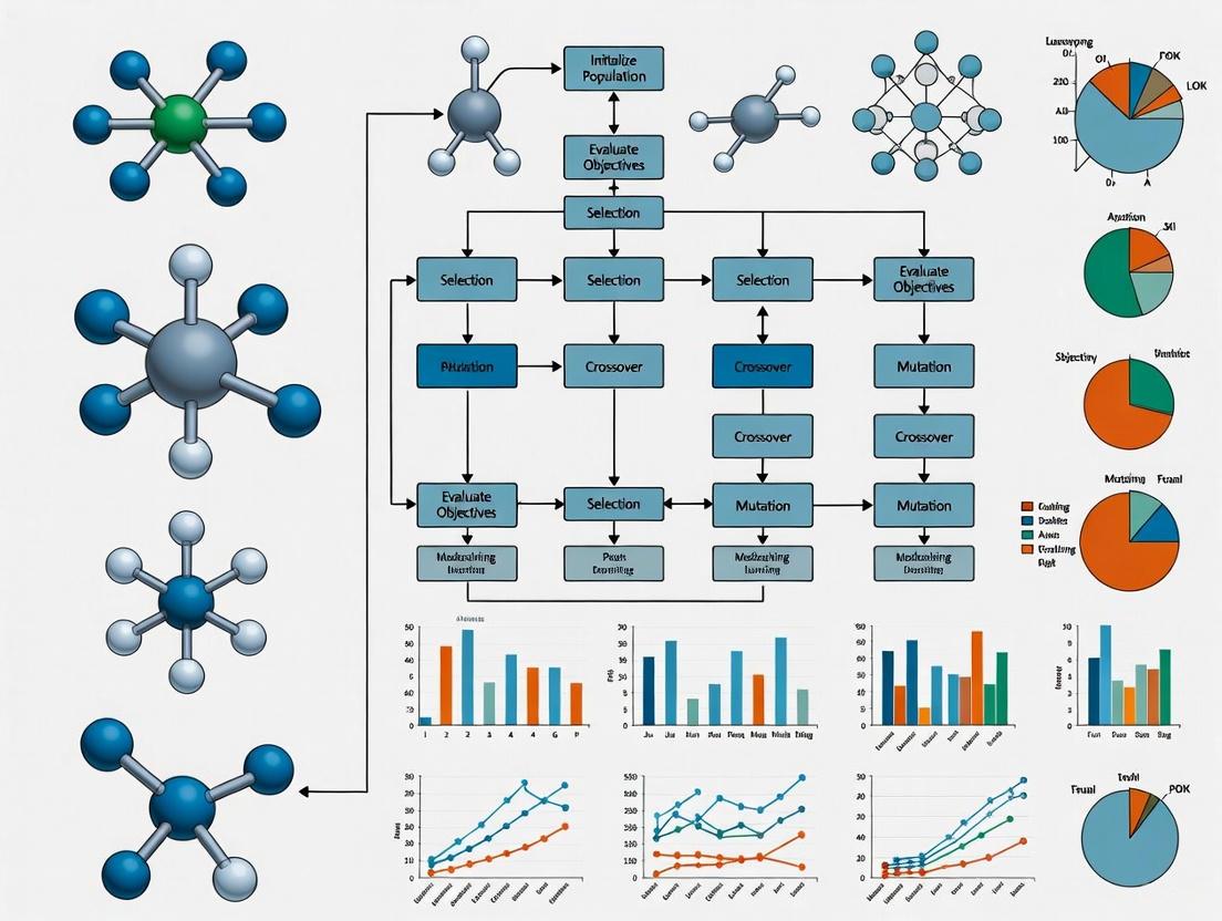
The following diagram illustrates a generalized workflow for conducting multi-objective optimization studies, particularly relevant for EMO research:
Multi-Objective Optimization Workflow
The Scientist's Toolkit: Research Reagent Solutions
Table: Essential Computational Tools for Multi-Objective Optimization Research
| Tool Category | Representative Examples | Function in MOO Research |
|---|---|---|
| Optimization Frameworks | OpenMDAO [2], PlatEMO, jMetal | Provide infrastructure for implementing and testing MOO algorithms |
| Benchmark Problems | ZDT, DTLZ, WFG test suites | Standardized problems for comparing algorithm performance |
| Performance Indicators | Hypervolume, Generational Distance, Inverted Generational Distance | Quantify convergence and diversity of obtained solutions |
| Visualization Tools | Pareto front plots, parallel coordinate plots, heat maps | Enable interpretation of high-dimensional optimization results |
| Multi-Criteria Decision Making | AHP (Analytic Hierarchy Process), TOPSIS | Support selection of final solution from Pareto optimal set |
Applications in Research and Industry
Multi-objective optimization has been applied across numerous fields, demonstrating its versatility in addressing complex real-world problems [1]:
- Engineering Design: Balancing performance, cost, and reliability in aerospace, automotive, and structural design [2]
- Economics and Finance: Portfolio optimization to maximize returns while minimizing risk [1]
- Process Optimization: Chemical engineering and manufacturing processes with conflicting objectives like yield, purity, and energy consumption [1]
- Drug Development: Optimizing therapeutic efficacy while minimizing side effects and production costs
The continuing development of EMO algorithms addresses increasingly complex problems across these domains, with current research focusing on scaling to higher-dimensional problems, incorporating machine learning techniques, and improving computational efficiency [3] [4].
Evolutionary Multi-objective Optimization (EMO) research addresses problems where multiple, often conflicting, objectives must be simultaneously optimized. In such problems, improving one objective typically leads to deterioration in another, creating a complex landscape of trade-offs. The Pareto principle provides the foundational theory for understanding and solving these multi-objective problems. It defines Pareto optimality as a state where no objective can be improved without worsening at least one other objective [5]. The set of all Pareto optimal solutions forms the Pareto front (or Pareto frontier), which represents the complete spectrum of optimal trade-offs between competing objectives [5].
Within EMO research, the primary goal is to develop algorithms that can efficiently approximate the true Pareto front of a problem, providing decision-makers with a comprehensive set of alternative solutions. This field has grown significantly from its origins, now encompassing sophisticated evolutionary and population-based algorithms, surrogate models, and hybrid machine learning methods [3]. The ensuing sections explore the theoretical foundations of Pareto optimality, computational methods for identifying Pareto fronts, and their critical applications in scientific domains such as drug development and chemical engineering.
Theoretical Foundations of Pareto Optimality and Frontiers
Formal Definition and Key Concepts
In multi-objective optimization, a system is defined by a function ( f: X \rightarrow \mathbb{R}^m ) that maps a decision variable ( x ) in the space ( X \subseteq \mathbb{R}^n ) to a vector of ( m ) objective values in ( \mathbb{R}^m ) [5]. The Pareto frontier, denoted as ( P(Y) ), where ( Y = {y \in \mathbb{R}^m: y = f(x), x \in X} ), is formally described as follows [5]:
[ P(Y) = { y' \in Y : { y'' \in Y : y'' \succ y', y' \neq y'' } = \emptyset }. ]
This means a point ( y' ) belongs to the Pareto front if no other point ( y'' ) dominates it. Domination (( y'' \succ y' )) occurs when ( y'' ) is at least as good as ( y' ) in all objectives and strictly better in at least one [5]. The Pareto frontier distinguishes acceptable compromises from suboptimal solutions that can be objectively improved [6].
Marginal Rate of Substitution in Pareto Efficiency
A significant aspect of the Pareto frontier in economics and beyond is that at any Pareto-efficient allocation, the marginal rate of substitution (MRS) is identical across all consumers or objectives [5]. For a system with ( m ) consumers and ( n ) goods, this implies:
[ \frac{f{xj^i}^{i}}{f{xs^i}^{i}} = \frac{\muj}{\mus} = \frac{f{xj^k}^{k}}{f{xs^k}^{k}}. ]
Here, ( f{xj^i} ) represents the partial derivative of the utility function ( f ) with respect to good ( j ) for consumer ( i ), and ( \muj ) and ( \mus ) are Lagrange multipliers associated with the constraints on goods ( j ) and ( s ) [5]. This equality shows that in a Pareto-optimal state, the rate at which any consumer is willing to trade one good for another is uniform, indicating an efficient allocation of resources where no reallocation can improve one individual's situation without harming another's.
Computational Methods for Pareto Frontier Identification
Computing the Pareto frontier is a central challenge in EMO. Algorithms must find a set of solutions that are both diverse and close to the true Pareto front. The following table summarizes core computational approaches used in EMO research.
Table 1: Algorithms for Computing and Approximating the Pareto Front
| Algorithm Type | Core Principle | Key Advantages | Common Applications |
|---|---|---|---|
| Scalarization (Weighted Sum) [5] | Transforms multi-objective problem into a single objective using a weighted sum of objectives. | Simple to implement; intuitive. | Convex Pareto fronts; preliminary analysis. |
| ε-Constraint Method [5] | Optimizes one primary objective while treating others as constraints with ε thresholds. | Can find solutions on non-convex parts of the Pareto front. | Problems with non-convex Pareto fronts. |
| Multi-objective Evolutionary Algorithms (MOEAs) [5] [3] | Uses population-based search (e.g., selection, crossover, mutation) to approximate the front in a single run. | Finds diverse sets of solutions in parallel; handles complex, non-linear landscapes. | Complex black-box problems; engineering design. |
| Machine Learning / Bayesian Optimization [7] | Builds surrogate models (e.g., Gaussian Processes) to guide the search efficiently. | Highly data-efficient; suitable for expensive objective functions (e.g., chemical experiments). | Automated chemistry; reaction optimization. |
| Skyline Query / Maxima of a Point Set [5] | Directly compares vectors to filter out dominated solutions from a finite set. | Effective for pre-computed datasets or low-dimensional spaces. | Database queries; decision support systems. |
For complex or computationally expensive problems, generating the entire Pareto front can be intractable. Therefore, approximation algorithms are employed. An ε-approximation of a Pareto front ( P ) is a set ( S ) where the directed Hausdorff distance between ( S ) and ( P ) is at most ( ε ), requiring roughly ( (1/ε)^d ) queries for a ( d )-dimensional problem [5]. The performance of these approximations is evaluated based on criteria like invariance to scaling, monotonicity, and computational complexity [5].
The following diagram illustrates a high-level workflow for a machine learning-driven multi-objective optimization, as used in fields like automated chemistry.
Experimental Protocols and Applications
Detailed Protocol: Multi-Objective Optimization in Continuous Flow Chemistry
A seminal application of EMO principles in experimental science is the automated optimization of chemical reactors using machine learning [7]. The following protocol details the methodology.
- Objective: To simultaneously optimize conflicting performance criteria—specifically, reactor productivity (an economic objective) and environmental impact (an environmental objective)—for chemical reactions in a continuous flow reactor [7].
- Algorithm: A multi-objective machine learning algorithm (e.g., based on Gaussian Process models) was implemented for self-optimization [7].
- Procedure:
- Initialization: The algorithm is initiated with a small set of initial experiments that sample the parameter space (e.g., reactant concentration, flow rate, temperature).
- Modeling: A Gaussian Process (GP) surrogate model is constructed to approximate the relationship between the input parameters and the multiple objective functions. This model provides predictions of performance and associated uncertainty for untested parameters [7].
- Iteration: a. Selection: An acquisition function, guided by the GP model, selects the next set of reactor parameters to evaluate. This function balances exploring uncertain regions and exploiting known high-performance areas. b. Experiment: The selected parameters are automatically executed in the continuous flow reactor system. c. Evaluation: The productivity and environmental impact (e.g., E-factor, energy consumption) of the reaction are measured. d. Update: The GP model is updated with the new experimental results.
- Termination: The loop continues until a predefined budget of experiments is exhausted or the Pareto front is sufficiently well-defined.
- Outcome: The algorithm successfully identifies the Pareto front, visually represented as a trade-off curve between the environmental and economic objectives. This reveals all optimal compromises, showing that increasing productivity requires a concession in environmental performance, and vice versa [7]. The machine learning approach proved highly data-efficient, achieving optimization in fewer experiments than single-objective approaches [7].
The Scientist's Toolkit: Key Reagents and Materials
The following table details essential components for setting up an automated optimization system for chemical synthesis, as described in the protocol.
Table 2: Research Reagent Solutions for Automated Reaction Optimization
| Item Name | Function / Explanation |
|---|---|
| Continuous Flow Reactor | A reactor where reactants are continuously pumped through a reaction channel. Essential for precise parameter control and automation, enabling rapid experimentation [7]. |
| Gaussian Process Model | A probabilistic machine learning model. Serves as a surrogate for expensive experiments, predicting reaction outcomes and their uncertainty based on input parameters [7]. |
| Multi-Objective Acquisition Function | The decision-making engine (e.g., based on Expected Hypervolume Improvement). Uses the surrogate model to select the most informative parameters to test next, balancing multiple goals [7]. |
| Precursor Chemicals | The specific reactants for the synthesis being optimized. Their concentrations and ratios are key variables in the optimization process. |
| In-line Analytical Sensors | Sensors (e.g., IR, UV-Vis) integrated into the flow system. Provide real-time data on reaction conversion and selectivity, enabling immediate evaluation of objectives [7]. |
Application in Pharmaceutical Development
The Pareto principle finds critical application in pharmacoepidemiology for enhancing drug therapy safety. A study investigating adverse drug events (ADE) and medication errors (ME) in an emergency department (ED) demonstrated its utility [8].
- Methodology: Researchers analyzed 752 consecutive cases admitted to a non-traumatic ED. ADEs, MEs, contributing drugs, preventability, and detection rates were recorded. Symptoms, errors, and drugs were sorted by frequency to apply the Pareto principle [8].
- Findings: The study identified 242 ADEs, 61.2% of which were preventable. A limited subset of factors was responsible for the majority of outcomes:
- The ten most frequent symptoms accounted for 80% of ADE-related hospitalizations [8].
- A set of only 33 drugs was responsible for 76% of all ADEs [8].
- This frequency-based listing allowed researchers to identify the most locally relevant problems and develop targeted safety interventions, such as wall and pocket charts for ED staff [8].
This application highlights how Pareto analysis can efficiently direct limited resources toward the most impactful factors in complex healthcare systems.
Visualization and Analytical Tools
The Pareto Chart for the 80-20 Rule
A Pareto chart is a specialized bar chart that visualizes the Pareto principle (or the 80-20 rule), which states that a small percentage of factors often contribute to a large percentage of the effects [9]. It is used extensively in quality control and process improvement.
- Construction:
- Data Preparation: Categories (e.g., types of defects, complaint issues) are sorted in descending order by their frequency or cost.
- Cumulative Percentage: A line is added to the chart showing the cumulative percentage of the total as each category is added.
- Interpretation: The chart helps identify the "vital few" categories that, if addressed, would resolve the bulk of the problems. For example, an analysis of consumer complaints showed that the top 20% of issue types generated over 80% of all complaints [9].
The diagram below illustrates the logical structure of a system designed to help users navigate the Pareto frontier in an exploratory search context, such as e-commerce or research databases.
The Pareto principle and the concept of the Pareto frontier provide an essential framework for tackling complex, multi-objective problems across science and engineering. Within Evolutionary Multi-Objective Optimization research, the focus is on developing sophisticated algorithms—from evolutionary methods to machine learning hybrids—to efficiently approximate this frontier. As demonstrated by applications in automated chemistry and drug safety, moving beyond single-objective optimization to a holistic trade-off analysis is crucial for informed decision-making. The ongoing integration of EMO with artificial intelligence and adaptive interactive systems promises to further empower researchers and professionals in navigating the intricate landscape of competing objectives.
Evolutionary Algorithms as a Solution Strategy for Complex Problems
Evolutionary Multi-Objective Optimization (EMO) represents a specialized class of evolutionary algorithms that tackle problems with multiple, often conflicting, objectives. Unlike single-objective optimization, which converges toward a single solution, EMO algorithms identify a set of optimal solutions, known as the Pareto-optimal front. This front illustrates the trade-offs between objectives, enabling decision-makers to select the most appropriate solution based on their specific requirements. The 13th International Conference on Evolutionary Multi-Criterion Optimization (EMO 2025) highlights the continued advancement of this field, with proceedings covering algorithm design, benchmarking, applications, and multi-criteria decision support [4].
EMO research is particularly valuable for complex, real-world problems where no single perfect solution exists. By leveraging population-based search inspired by natural evolution, EMO algorithms can explore diverse regions of the search space simultaneously and approximate the entire Pareto-optimal front in a single run. This capability makes them exceptionally suited for challenging domains such as drug development, where researchers must balance efficacy, toxicity, cost, and other critical factors simultaneously.
Core Algorithmic Frameworks in EMO
Fundamental EMO Algorithm Design
EMO algorithms combine evolutionary computation principles with specialized mechanisms for handling multiple objectives. Most modern EMO approaches incorporate three key components: fitness assignment that reflects multiple objectives, diversity preservation mechanisms to maintain a spread of solutions along the Pareto front, and elitism to retain high-quality solutions across generations. The field has evolved from early non-elitist methods like VEGA and MOGA to sophisticated elitist algorithms such as NSGA-II, SPEA2, and more recent metric-based and decomposition-based approaches.
Key hybrid approaches are also emerging, as evidenced by research presented at EMO 2025. One paper describes "An MaOEA/Local Search Hybrid Based on a Fast, Stochastic BFGS Using Achievement Scalarizing Search Directions," which combines multi-objective evolutionary algorithms with local search refinement for improved performance [4]. Another contribution, "MOAISDX: A New Multi-objective Artificial Immune System Based on Decomposition," demonstrates how biological inspiration beyond natural selection can inform algorithm design [4].
EMO Algorithm Workflow
The following diagram illustrates the generalized workflow of an evolutionary multi-objective optimization algorithm:
Benchmarking and Performance Assessment
Robust benchmarking is essential for advancing EMO research. The "MO-IOHinspector: Anytime Benchmarking of Multi-objective Algorithms Using IOHprofiler" presented at EMO 2025 addresses this need by providing comprehensive tools for performance tracking across different stages of the optimization process [4]. Benchmarking in EMO requires specialized performance indicators that evaluate both convergence to the true Pareto-optimal front and diversity of solutions along the front. Common metrics include:
Table 1: Key Performance Metrics for EMO Algorithms
| Metric | Purpose | Interpretation |
|---|---|---|
| Hypervolume (HV) | Measures the volume of objective space dominated by solutions | Higher values indicate better convergence and diversity |
| Inverted Generational Distance (IGD) | Computes average distance from reference Pareto front to obtained solutions | Lower values indicate better convergence to the true front |
| Spread (Δ) | Quantifies the diversity and distribution of solutions | Lower values indicate more uniform distribution along the front |
| Epsilon (ε) Indicator | Measures the smallest factor needed to transform obtained set to dominate reference set | Lower values indicate better quality approximation sets |
EMO Applications in Scientific and Industrial Domains
Drug Development Applications
EMO algorithms offer significant advantages in pharmaceutical research, where multiple competing objectives must be balanced simultaneously. In drug discovery, these algorithms can optimize molecular structures to maximize therapeutic efficacy while minimizing toxicity, side effects, and production costs. The multi-objective approach allows medicinal chemists to explore the complex trade-off landscape and identify promising candidate molecules worthy of further experimental investigation.
Specific applications in drug development include:
- Molecular Design: Simultaneously optimizing binding affinity, solubility, metabolic stability, and synthetic accessibility
- Clinical Trial Design: Balancing statistical power, patient recruitment feasibility, cost constraints, and ethical considerations
- Formulation Optimization: Maximizing drug stability, bioavailability, and manufacturability while minimizing excipient costs
- Treatment Scheduling: Optimizing dosage regimens for efficacy, reduced side effects, and minimized development of drug resistance
Free-Form Coverage Path Planning
The EMO 2025 proceedings include research on "Encodings for Multi-objective Free-Form Coverage Path Planning," demonstrating how EMO approaches solve complex spatial optimization problems with applications in areas ranging from robotic surgery to agricultural automation [4]. This work highlights the importance of specialized solution representations tailored to specific problem domains, a recurring theme in successful EMO applications.
Experimental Protocols and Methodologies
Standard Experimental Framework for EMO Research
Conducting rigorous EMO experiments requires careful methodology to ensure valid, reproducible results. The following protocol outlines a comprehensive approach for evaluating EMO algorithm performance:
Phase 1: Problem Formulation
- Objective Definition: Clearly specify all objective functions to be optimized, noting any conflicts between objectives.
- Constraint Identification: Define all problem constraints and determine appropriate constraint-handling mechanisms (penalty functions, feasibility rules, etc.).
- Decision Variable Encoding: Establish suitable representation for decision variables (binary, real-valued, permutation, etc.) based on problem structure.
Phase 2: Experimental Setup
- Algorithm Configuration: Set population size, termination criteria (maximum generations, function evaluations, or convergence thresholds), and operator parameters (crossover and mutation rates).
- Benchmark Selection: Choose appropriate test problems with known Pareto-optimal fronts, spanning different characteristics (concave, convex, disconnected, multimodal).
- Performance Metrics: Select relevant quality indicators (see Table 1) aligned with research objectives.
Phase 3: Execution and Analysis
- Multiple Independent Runs: Execute algorithm multiple times (typically 20-30 runs) with different random seeds to account for stochastic variations.
- Statistical Testing: Apply appropriate statistical tests (Wilcoxon signed-rank, Kruskal-Wallis) to determine significance of performance differences.
- Visualization: Generate Pareto front approximations, performance trajectories, and comparative plots to facilitate interpretation.
Research Reagent Solutions for EMO Experimentation
Table 2: Essential Computational Tools for EMO Research
| Tool/Category | Function | Examples/Alternatives |
|---|---|---|
| Optimization Frameworks | Provides implementations of EMO algorithms | Platypus, jMetal, pymoo, DEAP |
| Benchmark Suites | Standardized test problems for algorithm comparison | ZDT, DTLZ, WFG test problems |
| Performance Assessment Tools | Calculate quality indicators and generate comparisons | METCO Library, IOHprofiler [4] |
| Visualization Libraries | Generate 2D/3D plots of Pareto fronts and performance metrics | Matplotlib, Plotly, ParaView |
| Statistical Analysis Packages | Perform significance testing and result analysis | SciPy, R, Statistica |
| High-Performance Computing | Enable computationally intensive EMO applications | MPI, OpenMP, GPU computing frameworks |
Advanced Methodologies and Hybrid Approaches
Integration with Machine Learning and Surrogates
A significant trend in EMO research involves combining evolutionary algorithms with machine learning techniques, particularly surrogate modeling. As indicated in the EMO 2025 proceedings, surrogates and machine learning approaches help address one of the fundamental challenges in EMO: the computational expense of evaluating objective functions, especially for real-world problems where each evaluation might involve complex simulations or physical experiments [4].
Surrogate-assisted EMO approaches typically follow this workflow:
- Initial Sampling: Design an initial experimental design to populate the surrogate training set
- Model Building: Construct approximate models of the objective functions using techniques like Kriging, radial basis functions, or neural networks
- Infill Criteria: Balance exploration and exploitation when selecting new points for expensive evaluation
- Model Update: Iteratively refine surrogates as new data becomes available
Multi-Criteria Decision Support Systems
EMO 2025 highlights the importance of "Multi-criteria decision support" as a key research topic, recognizing that identifying the Pareto-optimal front is only part of the solution process [4]. Effective decision support systems help stakeholders navigate the trade-off surface and select the most appropriate solution based on their preferences. These systems may incorporate:
- Preference Elicitation Methods: Techniques to capture and model decision-maker preferences
- Interactive EMO Approaches: Algorithms that incorporate decision-maker feedback during the optimization process
- Visual Analytics Tools: Advanced visualization techniques for exploring high-dimensional Pareto fronts
- Robust Decision Making: Methods for selecting solutions that perform well across different scenarios or in the presence of uncertainty
The following diagram illustrates the structure of a surrogate-assisted EMO framework with decision support:
Future Directions in EMO Research
The EMO 2025 conference proceedings indicate several emerging research directions that will shape the future of evolutionary multi-objective optimization. These include:
- Many-Objective Optimization: Developing scalable algorithms for problems with four or more objectives, where traditional Pareto-based approaches face challenges
- Expensive Optimization Problems: Advancing surrogate modeling and model management techniques for problems with computationally intensive evaluations
- Dynamic and Uncertain Environments: Creating algorithms that can adapt to changing environments and handle various forms of uncertainty
- Parallel and Distributed EMO: Leveraging high-performance computing architectures to solve increasingly complex problems
- Real-World Applications: Transferring EMO methodologies to challenging domains including personalized medicine, renewable energy systems, and sustainable engineering design
As EMO research continues to evolve, the integration of evolutionary computation with machine learning, decision science, and domain-specific knowledge will further establish evolutionary algorithms as a powerful solution strategy for complex, multi-objective problems across scientific and industrial domains.
Evolutionary Multiobjective Optimization (EMO) represents a subfield of computational intelligence that uses evolutionary algorithms to solve problems with multiple, often conflicting, objectives [10]. These multi-objective optimization problems (MOPs) yield a set of optimal solutions known as the Pareto set, with their images in the objective space forming the Pareto front [10]. Traditionally, EMO research has focused on problems with two or three objectives, where algorithms such as NSGA-II, SPEA2, and MOEA/D have demonstrated remarkable success [11].
However, many real-world problems involve concurrent optimization of numerous objectives. When the number of objectives exceeds three, these are classified as many-objective optimization problems [11]. This scaling introduces fundamental challenges that have necessitated new algorithmic paradigms and theoretical frameworks within EMO research. The transition from EMO to many-objective optimization represents a significant evolution in the field, driven by practical applications and addressing core computational challenges including selection pressure, diversity maintenance, and computational complexity [11].
Fundamental Challenges in Many-Objective Optimization
Core Algorithmic Difficulties
Scaling evolutionary algorithms to many objectives presents several interconnected challenges that distinguish this domain from traditional EMO research.
Pareto Dominance Degradation: As the number of objectives increases, the proportion of non-dominated solutions in a randomly generated population grows exponentially [11]. This erosion of selection pressure severely impedes convergence toward the true Pareto front, as the search process lacks sufficient guidance to distinguish superior solutions [11].
Visualization and Decision-Making Complexity: While EMO researchers have developed effective visualization techniques for two and three-dimensional objective spaces, visualizing high-dimensional Pareto fronts for many-objective problems remains challenging [11]. This complicates both algorithm development and decision-making processes.
Computational Resource Demands: The assessment of solution quality in many-objective spaces often requires computationally intensive indicators such as hypervolume [11]. Additionally, maintaining diverse solution sets across high-dimensional fronts necessitates larger population sizes and archive mechanisms, further increasing computational costs [11].
Performance Assessment in High-Dimensional Spaces
Traditional performance indicators used in EMO require adaptation or replacement for many-objective optimization. The table below summarizes key indicators and their applicability to many-objective problems.
Table 1: Performance Indicators for Many-Objective Optimization
| Indicator | Primary Function | Scalability to Many Objectives | Computational Cost |
|---|---|---|---|
| Hypervolume | Measures dominated volume | Good, but becomes expensive | High, grows with objectives and population |
| IGD (Inverted Generational Distance) | Measures convergence and diversity | Good with true Pareto front reference | Moderate, depends on reference set size |
| R2 Indicator | Uses utility functions | Good, more scalable than hypervolume | Low to moderate |
| Hausdorff Distance | Measures distance between sets | Moderate, can be sensitive to outliers | Moderate |
| Solow-Polasky Diversity | Measures solution diversity | Good for diversity-focused optimization | Moderate, involves matrix calculations |
Algorithmic Approaches for Many-Objective Optimization
Dominance-Based Modifications
Researchers have developed several strategies to address dominance degradation in many-objective optimization:
Relaxed Dominance Criteria: Approaches such as ε-dominance, cone dominance, and fuzzy dominance expand the dominance area to facilitate better solution discrimination [11]. These methods help restore selection pressure by making dominance relationships more likely.
Reference Point-Based Methods: Algorithms like NSGA-III use reference points supplied by decision makers to maintain population diversity across high-dimensional objective spaces [11]. This approach shifts focus from Pareto dominance to reference-driven diversity maintenance.
Indicator-Based Selection: Hypervolume-based algorithms and other indicator-based approaches replace Pareto dominance with quality indicators directly in the selection process [11]. While computationally demanding, these methods provide explicit optimization goals.
Decomposition and Dimension Reduction
Objective Reduction Techniques: These approaches identify redundant objectives that can be eliminated without substantially altering the problem structure, effectively reducing a many-objective problem to one with fewer objectives [11].
Aggregation Methods: Weighted sum approaches and other aggregation methods combine multiple objectives into a single fitness function, though this may obscure trade-off information [11].
Evolutionary Multitasking: A novel paradigm exemplified by the EMCMOA algorithm, which decomposes complex constrained many-objective problems into interdependent tasks [12]. The framework employs a dual-task structure where a helper task addresses unconstrained objective optimization and transfers knowledge to the main task focused on constraint satisfaction [12].
Table 2: Comparison of Many-Objective Optimization Algorithms
| Algorithm | Core Mechanism | Scalability | Constraint Handling | Key Advantages |
|---|---|---|---|---|
| NSGA-III | Reference point-based | Good for 3-15 objectives | Requires extension | Maintains diversity in high-dimensional spaces |
| MOEA/D | Decomposition | Good for many objectives | Requires extension | Leverages single-objective optimizers |
| SPEA2 | Improved fitness assignment | Moderate (2-5 objectives) | Requires extension | Effective archive strategy |
| EMCMOA | Evolutionary multitasking | Good for constrained problems | Native constraint handling | Knowledge transfer between tasks [12] |
| HypE | Hypervolume approximation | Good for many objectives | Requires extension | Scalable hypervolume estimation |
Experimental Protocols and Benchmarking
Standard Test Problems
Researchers typically evaluate many-objective optimization algorithms using scalable test suites that allow controlled assessment of algorithmic performance:
DTLZ Test Suite: The DTLZ (Deb-Thiele-Laumanns-Zitzler) problem family provides scalable test problems with known Pareto fronts, enabling systematic evaluation of convergence and diversity properties [11].
WFG Toolkit: The WFG (Walking Fish Group) test problems feature more complex Pareto set shapes and include position-related parameters that complicate optimization [11].
Performance Evaluation Methodology
Comprehensive algorithm assessment follows standardized experimental protocols:
Algorithm Configuration: Multiple population sizes (typically 36-210 individuals) are tested under fixed evaluation budgets [13]. Smaller populations may be sufficient when using external archives [13].
Performance Metrics Calculation: Algorithms are evaluated using quality indicators including:
- Inverted Generational Distance (IGD) measuring convergence and diversity
- Hypervolume (HV) measuring dominated space
- Δp indicator for completeness of Pareto front coverage [13]
Statistical Validation: Results are statistically compared using non-parametric tests like Wilcoxon signed-rank test with Bonferroni correction to ensure significance [12].
Constraint Handling Assessment: For constrained problems, algorithms are evaluated on both artificial and real-world problems to identify performance differences across problem types [13].
Research Toolkit for Many-Objective Optimization
Table 3: Essential Research Tools and Resources
| Tool/Resource | Type | Primary Function | Application Context |
|---|---|---|---|
| JMetal | Software Framework | Algorithm implementation | Rapid prototyping of EMO algorithms |
| PlatEMO | Software Platform | Integrated EMO environment | Algorithm benchmarking and comparison |
| DTLZ/WFG | Test Problems | Algorithm performance assessment | Controlled experimental studies |
| Hypervolume | Performance Indicator | Solution quality measurement | Algorithm validation and comparison |
| EMCMOA | Algorithm | Constrained many-objective optimization | Real-world problems with constraints [12] |
Visualization of Algorithm Frameworks
The following diagram illustrates the core structure of an evolutionary multitasking framework for many-objective optimization, as implemented in the EMCMOA algorithm:
Figure 1: EMCMOA Evolutionary Multitasking Framework
The EMCMOA algorithm implements a dual-task structure where knowledge transfer between constrained and unconstrained optimization tasks enhances search efficiency [12]. This framework demonstrates how decomposition and knowledge sharing can address complex constrained many-objective optimization problems.
Application Case Study: Reservoir Scheduling
A practical application of many-objective optimization is found in cascade reservoir scheduling for small watersheds, which must balance multiple competing objectives [12]. The Lushui River Basin case study demonstrates a real-world implementation with the EMCMOA algorithm achieving up to 15.7% improvement in IGD and 12.6% increase in HV compared to state-of-the-art algorithms [12].
The many-objective scheduling model incorporates five critical objectives:
- Flood Control: Minimize peak water levels during precipitation events
- Ecological Water Requirements: Maintain minimum flow rates for ecosystem health
- Hydropower Generation: Maximize energy production from reservoir systems
- Agricultural Irrigation: Meet seasonal water demands for crop cultivation
- Industrial Water Supply: Ensure reliable water access for industrial operations
This application highlights the practical necessity of many-objective optimization approaches for complex real-world systems with numerous competing demands [12].
Future Research Directions
The field of many-objective optimization continues to evolve with several promising research trajectories:
Integration with Machine Learning: Surrogate modeling and Bayesian optimization techniques show potential for reducing computational costs in many-objective optimization [3] [13].
Theoretical Foundations: Enhanced understanding of search space characteristics and problem dimensionality effects will inform more robust algorithm design [10].
Interactive Optimization: Incorporating decision-maker preferences during the optimization process rather than as a post-processing step [10].
Scalable Visualization Techniques: Developing effective methods for visualizing and interpreting high-dimensional Pareto fronts to support decision-making [11].
The progression from EMO to many-objective optimization represents a natural maturation of the field, addressing increasingly complex real-world problems while developing sophisticated computational approaches to manage the challenges of high-dimensional objective spaces.
EMO Algorithms and Breakthrough Applications in Biomedicine and Drug Design
Many real-world problems in science and engineering, including those in drug development and complex system design, require the simultaneous optimization of several conflicting objectives. These are known as Multi-objective Optimization Problems (MOPs). Unlike single-objective problems, MOPs do not have a single optimal solution but instead a set of optimal trade-off solutions, collectively known as the Pareto-optimal front. Evolutionary Multi-objective Optimization (EMO) algorithms are a class of population-based stochastic search methods that are particularly well-suited for solving MOPs, as they can approximate the entire Pareto front in a single run. Within EMO research, dominance-based algorithms form a foundational pillar. These algorithms use the concept of Pareto dominance to compare and select solutions without requiring prior weighting of objectives. Among them, the Non-dominated Sorting Genetic Algorithm II (NSGA-II) and the Strength Pareto Evolutionary Algorithm 2 (SPEA2) are two of the most widely used and cited algorithms. This whitepaper provides an in-depth technical guide to their core mechanisms, performance, and applications, situating them within the broader context of modern EMO research.
Foundational Concepts and Definitions
Pareto Dominance and Optimality
- Pareto Dominance: A solution x is said to dominate a solution y (denoted x ≺ y) if two conditions are met:
- The solution x is no worse than y in all objectives.
- The solution x is strictly better than y in at least one objective.
- Pareto-Optimal Set: The set of all solutions in the decision variable space that are non-dominated by any other solution in the feasible space.
- Pareto Front (PF): The image of the Pareto-optimal set in the objective space, representing the set of optimal trade-offs.
Core Goals of EMO Algorithms
The primary goals of an EMO algorithm are:
- Convergence: The population of solutions should converge towards the true Pareto-optimal front.
- Diversity: The solutions should be well-spread and diverse across the Pareto front to provide the decision-maker with a rich set of alternatives.
The NSGA-II Algorithm
Core Mechanism
NSGA-II employs a three-step mechanism to achieve convergence and diversity [14].
- Non-dominated Sorting: The population is hierarchically classified into a sequence of non-dominated fronts (Front 1, Front 2, ..., Front k). Front 1 contains all non-dominated solutions in the current population; after removing these, Front 2 contains the next set of non-dominated solutions, and so on. This sorting provides the primary convergence pressure towards the Pareto front.
- Crowding Distance Assignment: Within each front, a density estimation metric is calculated for each solution. The crowding distance is the average side-length of the cuboid formed by a solution's immediate neighbors in the objective space. A larger crowding distance indicates a less crowded region and is preferred. This metric promotes diversity.
- Elitist Selection: The algorithm combines the parent and offspring populations. It then selects the next generation by first choosing all solutions from the best non-dominated front (Front 1), then Front 2, and so on. When the last front to be included cannot be accommodated fully, the solutions within that front with the largest crowding distance are selected. This ensures elitism and diversity preservation.
Workflow and Structure
The following diagram illustrates the step-by-step workflow of the NSGA-II algorithm.
The SPEA2 Algorithm
Core Mechanism
SPEA2 addresses some perceived weaknesses of earlier algorithms by using a fine-grained fitness assignment strategy and a density-based archive [15].
- Strength and Raw Fitness: Each solution i in both the main population and an external archive is assigned a strength value S(i), representing the number of solutions it dominates. The raw fitness R(i) of a solution is then determined by the sum of the strength values of all solutions that dominate it. Lower raw fitness is better. This provides a strong convergence pressure.
- Density Estimation: To further distinguish between solutions with identical raw fitness, SPEA2 incorporates a density estimate. The density D(i) is calculated using the inverse of the distance to the k-th nearest neighbor (typically k = √(population size + archive size)). A closer neighbor implies a more crowded region, and a higher density value.
- Archive Truncation: The total fitness F(i) is the sum of raw fitness and density (F(i) = R(i) + D(i)). The algorithm maintains an archive of fixed size containing the non-dominated solutions from the combined population and archive. If the number of non-dominated solutions exceeds the archive size, a truncation operator is used. It iteratively removes the solution with the smallest distance to its k-th neighbor, recalculating distances after each removal to ensure diversity is maintained.
Workflow and Structure
The following diagram illustrates the step-by-step workflow of the SPEA2 algorithm.
Comparative Performance Analysis
Theoretical and Practical Performance
Theoretical and empirical studies have highlighted key differences in the performance and behavior of NSGA-II and SPEA2.
Theoretical Runtime and Population Dynamics: A key theoretical insight is that the selection mechanisms of NSGA-II and SPEA2 lead to different population dynamics. The crowding distance in NSGA-II can cause the population to concentrate in the middle of the Pareto front. In contrast, the selection of SPEA2, which considers distances to all other individuals, tends to distribute solutions more evenly across the Pareto front. Recent runtime analysis shows that SPEA2's performance is less sensitive to increases in population size. For complex problems like OneJumpZeroJump, SPEA2 can achieve a runtime of O(n^(k+1)) for a wider range of population sizes (μ, λ = O(n^k)), whereas NSGA-II's best guarantee is achieved only for a specific population size (μ = Θ(n)), making parameter tuning easier for SPEA2 [16].
Empirical Performance on Benchmarks and Applications:
Table 1: Comparative Algorithm Performance on Various Problems
| Problem Domain | Key Performance Metrics | Reported NSGA-II Performance | Reported SPEA2 Performance | Source |
|---|---|---|---|---|
| Next Release Problem (NRP) [Software Engineering] | Hypervolume (HV), Spread, Runtime | Best CPU run time across all test scales. | -- | [17] |
| Job-Shop Scheduling [Manufacturing] | Hypervolume, R2 Indicator | Less efficient compared to SPEA2 and IBEA. | Most efficient for the task; yields good distribution. | [15] |
| General Multi-objective Benchmarks (e.g., OneJumpZeroJump) | Expected Runtime | Θ(μn log n) for OneMinMax (highly dependent on population size). | O(n^2 log n) for OneMinMax (less dependent on population size). | [16] |
Detailed Experimental Protocol
To ensure reproducibility, the following outlines a standard experimental protocol for comparing EMO algorithms, as inferred from the cited literature [17] [15].
Algorithm Configuration:
- Initialization: Set population size (N), archive size (for SPEA2), crossover probability (P_c), mutation probability (P_m), and distribution indices for simulated binary crossover (SBX) and polynomial mutation.
- Stopping Criterion: Define a maximum number of generations or function evaluations.
Problem Instantiation:
- Test Problems: Select standard benchmark problems (e.g., ZDT, DTLZ, WFG) or a real-world problem like the Next Release Problem (NRP) or Job-Shop Scheduling.
- Data Sets: For applied studies, use real-world datasets (e.g., Eclipse, Gnome, Mozilla for NRP).
- Objective Functions: Clearly define the objective functions to be optimized (e.g., maximize customer satisfaction and minimize cost for NRP; minimize makespan, mean flow time, and variance for Job-Shop Scheduling).
Performance Measurement:
- Independent Runs: Execute each algorithm configuration for a statistically significant number of independent runs (e.g., 30 runs) to account for stochasticity.
- Quality Indicators: Calculate performance indicators for the final population/archive of each run.
- Hypervolume (HV): Measures the volume of objective space dominated by the solution set relative to a reference point. Higher HV indicates better convergence and diversity.
- Spread (Δ): Measures the extent of spread achieved among the obtained solutions. A lower value indicates a more uniform distribution.
- R2 Indicator: Measures the average distance of solutions to a utility function, reflecting convergence.
Data Analysis:
- Descriptive Statistics: Report the mean and standard deviation of the performance indicators across all runs.
- Statistical Testing: Perform non-parametric statistical tests (e.g., Wilcoxon rank-sum test) to determine if performance differences between algorithms are statistically significant.
The Scientist's Toolkit: Research Reagent Solutions
Table 2: Essential Components for EMO Algorithm Implementation and Evaluation
| Component / Tool | Function / Purpose | Example Use-Case |
|---|---|---|
| Standard Benchmark Suites (e.g., ZDT, DTLZ, WFG) | Provides a standardized set of test problems with known Pareto fronts to validate and compare algorithm performance. | Initial validation of a new NSGA-II variant's convergence on DTLZ2. |
| Performance Indicators (Hypervolume, Spread, R2) | Quantifiable metrics to assess the quality of an obtained solution set in terms of convergence and diversity. | Comparing the final archive of SPEA2 and NSGA-II on a scheduling problem using Hypervolume. |
| Statistical Testing Packages (e.g., in R or Python) | To perform rigorous statistical analysis of experimental results and confirm the significance of performance differences. | Using a Wilcoxon signed-rank test on Hypervolume values from 31 independent runs. |
| Reference Point (RP) | A vector in the objective space expressing a decision maker's preferences, used to guide the search towards a Region of Interest (ROI). | Integrating an RP into R-NSGA-II to find solutions near a specific cost-satisfaction trade-off in NRP. |
A significant trend in modern EMO research is the incorporation of decision-maker (DM) preferences to focus the search on a specific Region of Interest (ROI), thus improving scalability to many-objective problems. Both NSGA-II and SPEA2 have been extended in this context.
- Reference Point-Based NSGA-II (R-NSGA-II): This variant uses a supplied reference point to bias the selection process. Solutions closer to the reference point (measured by Euclidean distance) are preferred, leading the population to converge towards the ROI [14]. Recent modifications replace Euclidean distance with the Simplified Karush–Kuhn–Tucker Proximity Measure (S-KKTPM), which can predict convergence behavior without prior knowledge of the true Pareto front, yielding improved results [14].
- Preference-Based SPEA2: Concepts like g-dominance and r-dominance modify the Pareto dominance relation to incorporate preference information, allowing SPEA2 and similar algorithms to focus on the ROI [14].
NSGA-II and SPEA2 remain cornerstone algorithms in the field of evolutionary multi-objective optimization. While NSGA-II is often praised for its speed and effective use of elitism and crowding distance, SPEA2 offers a robust alternative with its fine-grained fitness assignment and archive truncation method, which can lead to more stable performance and better distribution, particularly on complex problems. The choice between them depends on the specific problem characteristics and the need for parameter robustness. The ongoing integration of preference information and theoretical runtime analysis continues to refine these classic algorithms, ensuring their relevance and application in solving complex, real-world optimization challenges in domains ranging from software engineering to drug development.
Evolutionary Multi-objective Optimization (EMO) research addresses problems with multiple conflicting objectives, known as Multi-objective Optimization Problems (MOPs). The core challenge lies in finding a set of optimal trade-off solutions rather than a single optimum [18]. Within this field, decomposition-based and indicator-based approaches represent two fundamental algorithmic philosophies for balancing convergence toward optimality with diversity across the Pareto front [18].
Multi-objective Evolutionary Algorithm based on Decomposition (MOEA/D), introduced by Zhang and Li in 2007, decomposes an MOP into multiple single-objective subproblems using scalarization functions and a set of weight vectors. These subproblems are then optimized simultaneously in a collaborative manner [19] [20]. In contrast, Indicator-based Multi-Objective Evolutionary Algorithms (IB-MOEAs) employ a performance indicator, such as Hypervolume, to guide the selection process, using this single metric to measure the quality of a solution set and drive the population toward both convergence and diversity [18].
This guide provides an in-depth technical examination of these two approaches, framing them within the broader context of EMO research. It details their core mechanisms, advanced variants, and practical applications, particularly in computationally expensive domains like drug design.
Foundational Principles of MOEA/D
Core Decomposition Framework
MOEA/D reformulates a multi-objective optimization problem into a collection of single-objective subproblems. Given an MOP to minimize ( F(x) = (f1(x), f2(x), \dots, fm(x)) ), MOEA/D employs a scalarization method to define ( N ) subproblems, each associated with a weight vector ( \lambda^i = (\lambda1^i, \dots, \lambdam^i) ) such that ( \sum{j=1}^m \lambdaj^i = 1 ) and ( \lambdaj^i \geq 0 ) [20]. The most common scalarization approaches are:
- Weighted Sum (WS): ( g^{ws}(x|\lambda) = \sum{j=1}^{m} \lambdaj f_j(x) ) [21]
- Weighted Tchebycheff (TCH): ( g^{te}(x|\lambda, z^) = \max_{1 \leq j \leq m} { \lambda_j | f_j(x) - z_j^ | } ) [19]
- Penalty-based Boundary Intersection (PBI): ( g^{pbi}(x|\lambda, z^) = d_1 + \theta d_2 ), where ( d_1 ) is the distance from ( F(x) ) to the ideal point ( z^ ) along the weight vector, and ( d_2 ) is the perpendicular distance to the weight vector; ( \theta ) is a preset penalty parameter [19]
The algorithm maintains a population of solutions, each corresponding to a subproblem. A key feature is the neighborhood relationship among subproblems, defined based on the proximity of their weight vectors. The reproduction of new solutions for each subproblem typically relies on information from its neighboring subproblems, which promotes convergence and maintains diversity [20].
Key Design Components and Challenges
The performance of MOEA/D hinges on several design components [20]:
- Weight Vector Settings: The initial distribution and potential adaptation of weight vectors significantly impact the diversity of solutions. Uniform sampling (e.g., via the Simplex Lattice Design) is common but may be ineffective for problems with irregular Pareto Fronts (PFs) [19].
- Sub-problem Formulations: The choice of scalarization function (WS, TCH, PBI) affects the algorithm's ability to handle different PF geometries, such as non-convex or disconnected fronts [19].
- Selection Mechanisms: Strategies for selecting solutions for reproduction and for survival into the next generation are crucial for balancing exploration and exploitation.
A major limitation of the original MOEA/D is its performance deterioration on MOPs with irregular POFs (e.g., disconnected, degenerate, or inverted) [19]. This is partly due to its geometric pattern of using a "single point and multiple directions," where the "single point" is the ideal or nadir point, and "multiple directions" are the preset weight vectors. This can cause solutions to concentrate in specific regions of the PF [19].
Advanced MOEA/D Variants and Methodologies
Adaptations for Irregular Pareto Fronts
Recent research has introduced significant improvements to overcome MOEA/D's limitations.
- Multiple Reference Points Strategy: One advanced variant replaces the "single point and multiple directions" approach with a framework of "multiple reference points and a single direction" [19]. This helps prevent the population from converging to a limited region of the PF. The algorithm includes methods for generating and adjusting these reference points during the evolutionary process to better match the true PF shape.
- Hybrid Decomposition Approaches: To tackle many-objective problems (those with 4+ objectives), MOEA/D-oDE combines the benefits of the Weighted Sum and Tchebycheff approaches. It uses an alterable decomposition method and incorporates optimal Differential Evolution (DE) schemes to enhance search capability [21].
- Adaptive Weight Vector Adjustment: MOEA/D-AWA periodically repairs the distribution of weight vectors by deleting vectors in crowded areas of the PF and generating new ones in sparse areas [19] [21]. This adaptive process allows the algorithm to dynamically respond to the evolving shape of the solution front.
Table 1: Advanced MOEA/D Variants and Their Core Improvements
| Variant Name | Core Improvement | Target Problem Type | Key Mechanism |
|---|---|---|---|
| MOEA/D with Multiple Reference Points [19] | Reference Point Geometry | Irregular POFs | Shifts from single ideal point to multiple reference points |
| MOEA/D-oDE [21] | Decomposition & Operator | Many-objective, Complex PFs | Hybrid WS/TCH decomposition; optimal DE schemes |
| MOEA/D-AWA [21] | Weight Vector Adaptation | General MOPs | Periodically deletes crowded/ adds sparse weight vectors |
| LSMOEA/D [22] | Decision Variable Analysis | Large-scale MaOPs | Integrates reference vectors for control variable analysis |
MOEA/D for Large-Scale and Many-Objective Problems
Large-scale high-dimensional many-objective optimization problems (LaMaOPs), characterized by numerous decision variables and objectives, present a substantial challenge. MOEA/D variants address these through:
- Decision Variable Analysis: LSMOEA/D incorporates reference vectors into the analysis of control variables, combining adaptive strategies to optimize high-dimensional decision spaces effectively [22].
- Cooperative Co-evolution: Some approaches break down the high-dimensional decision space into smaller components, optimizing them separately but cooperatively [22].
Foundational Principles of IB-MOEAs
Core Indicator-Based Framework
IB-MOEAs replace the traditional Pareto dominance-based selection with a performance indicator that evaluates the quality of a solution set. The core idea is to use this indicator directly as the selection criterion to drive the population toward the true Pareto front [18].
The most common environmental selection in IB-MOEAs is as follows [18]:
- A combined population ( Rt = Pt \cup Q_t ) (parents and offspring) is generated.
- The indicator value ( I({x}, A) ) is calculated for each solution ( x ) in ( R_t ), where ( A ) is a reference set (often the current population).
- Solutions are selected iteratively to form the next generation ( P_{t+1} ). In each iteration, the solution with the smallest indicator value is removed (minimizing the quality loss), until the population size reaches the desired size.
Key Indicators and Their Properties
The choice of indicator is critical, as different indicators balance convergence and diversity differently [18].
- Hypervolume (HV): Measures the volume of the objective space dominated by a solution set and bounded by a reference point. It is Pareto compliant, meaning that if a set A dominates set B, then A will have a higher hypervolume. It is considered a very comprehensive metric but is computationally expensive, especially as the number of objectives increases [18].
- Indicator ( I_{\epsilon+} ): A computationally efficient indicator that measures the minimum distance by which a solution set needs to be improved to dominate another set. It is less computationally intensive than hypervolume but can be biased toward convergence at the expense of diversity [18].
- ISDE+: An inverted version of the Shift-based Density Estimation indicator. It is computationally efficient and designed to consider both convergence and diversity simultaneously [18].
Table 2: Comparison of Common Indicators in IB-MOEAs
| Indicator | Pareto Compliant? | Computational Cost | Primary Bias | Key Advantage |
|---|---|---|---|---|
| Hypervolume (HV) | Yes | Very High (exponential in M) | Convergence & Diversity | Comprehensive quality measure |
| ( I_{\epsilon+} ) | No | Low | Convergence | Computational efficiency |
| ISDE+ | No | Low | Convergence & Diversity | Balanced performance; efficient |
Advanced IB-MOEAs and Hybrid Methodologies
Hybrid Selection MOEAs
Recognizing that different selection strategies have complementary strengths, recent research has focused on hybridization. The Hybrid Selection based MOEA (HS-MOEA) is one such algorithm that combines Pareto dominance, reference vectors, and an indicator [18].
HS-MOEA's environmental selection works as follows [18]:
- Pareto Dominance Filtering: The combined population is first sorted using non-dominated sorting. Solutions from the best non-dominated fronts are passed to the next stage.
- Reference Vector Assignment: The selected solutions are associated with predefined reference vectors to ensure diversity. Solutions are assigned to the reference vector with the smallest angle.
- Indicator-Based Final Selection: If a reference vector has more than one solution associated with it, the ISDE+ indicator is used to select the most suitable solution, ensuring both convergence and diversity within the niche.
This hybrid approach leverages the guaranteed convergence pressure of Pareto dominance, the diversity-preserving structure of reference vectors, and the fine-grained, balanced selection capability of an indicator.
Experimental Protocols and Performance Benchmarking
Standardized Testing and Evaluation Metrics
To validate and compare the performance of MOEA/D variants and IB-MOEAs, researchers employ standardized test suites and quality metrics.
- Test Suites: Common benchmark problems include the DTLZ and WFG test suites, which allow the configuration of various challenging PF characteristics such as convex, concave, disconnected, and degenerate shapes [18]. For large-scale problems, the LSMOP test suite is used [22].
- Performance Metrics:
- Inverted Generational Distance (IGD): Measures the average distance from the points in the true PF to the nearest solution in the approximated set. A lower IGD indicates better convergence and diversity [22].
- Hypervolume (HV): Measures the volume of the objective space dominated by the approximated set and bounded by a reference point. A higher HV indicates a better overall approximation of the PF [18].
Sample Experimental Protocol for Algorithm Comparison
A typical experimental protocol for benchmarking MOEAs involves the following steps [18]:
- Parameter Setup: Define the population size (e.g., 100 for 3-objective problems), termination condition (e.g., number of function evaluations), and other algorithm-specific parameters (e.g., neighborhood size in MOEA/D, penalty factor ( \theta ) in PBI).
- Independent Runs: Execute each algorithm a significant number of times (e.g., 20-30 independent runs) on each test instance to account for stochasticity.
- Data Collection: Record the final population from each run and calculate the performance metrics (IGD, HV) relative to the known true Pareto front.
- Statistical Analysis: Perform non-parametric statistical tests (e.g., the Wilcoxon rank-sum test) on the metric results to determine if performance differences between algorithms are statistically significant.
Application in Computer-Aided Drug Design
A prominent application of MOEAs is in Computer-Aided Drug Design (CADD), which aims to reduce the tremendous time and resource costs of developing new drugs by traversing the vast chemical space of potential compounds [23].
- Problem Formulation: The task is formulated as a multi-objective optimization problem where potential drug molecules (candidates) need to simultaneously optimize multiple properties, such as drug-likeness (QED), synthesizability (SA Score), and specific biological activities from benchmarks like GuacaMol [23].
- Algorithm Implementation: Studies have successfully deployed MOEAs like NSGA-II, NSGA-III, and MOEA/D for this purpose. A critical implementation detail is the molecular representation. While SMILES was traditionally used, the SELFIES representation is now preferred because it guarantees that every string corresponds to a valid molecular structure, leading to more efficient exploration [23].
- Outcome: Research results indicate that MOEAs show converging behavior and successfully optimize the defined criteria, discovering novel and promising candidate compounds for synthesis that are found in the obtained Pareto-sets [23].
Diagram 1: MOEA Workflow in Computer-Aided Drug Design
Table 3: Key Research Reagents and Computational Tools for EMO Research
| Item / Resource | Type | Primary Function in EMO Research |
|---|---|---|
| SELFIES [23] | Molecular Representation | String-based molecular representation guaranteeing 100% valid chemical structures for evolutionary operators. |
| GuacaMol Benchmark [23] | Benchmark Suite | Provides multi-objective tasks and metrics for benchmarking de novo molecular design algorithms. |
| DTLZ/WFG Test Suites [18] | Benchmark Problems | Standardized test problems for evaluating algorithm performance on various Pareto front geometries. |
| PlatEMO | Software Platform | An integrated MATLAB-based platform for experimental EMO research, featuring numerous algorithms. |
| Reference Vectors [18] | Algorithmic Component | A set of uniformly distributed vectors on a unit simplex used to guide diversity in RV-MOEAs and MOEA/D. |
| Hypervolume (HV) Calculator | Performance Metric | Software tool (e.g., in PyMOO) to compute the hypervolume indicator, measuring overall solution set quality. |
Diagram 2: Taxonomy of Multi-Objective Evolutionary Algorithm Frameworks
Decomposition-based (MOEA/D) and Indicator-based (IB-MOEAs) approaches represent two powerful and evolving paradigms within Evolutionary Multi-objective Optimization research. While MOEA/D offers a clear, decomposable structure and computational efficiency, IB-MOEAs provide a direct, quality-driven search guided by comprehensive performance metrics. The ongoing hybridization of these and other concepts, as seen in algorithms like HS-MOEA, demonstrates the field's dynamic nature and its continuous pursuit of more robust and effective optimization tools. The successful application of these algorithms in complex, real-world domains like computer-aided drug design underscores their significant practical value and potential for future impact across science and engineering.
Evolutionary Multi-objective Optimization (EMO) represents a class of population-based heuristic approaches for solving problems involving multiple conflicting objectives [24]. Traditional EMO algorithms aim to approximate the entire Pareto-optimal set, but as the number of objectives increases, this becomes computationally challenging and often impractical. Reference point methods address this limitation by incorporating decision maker (DM) preferences to focus the search on specific regions of interest (ROI) [14]. These methods enable a highly efficient search by allowing the DM to express preferences through desired objective values, guiding the optimization process toward solutions that better align with their expectations and requirements [25] [26].
The fundamental principle behind reference point methods is their ability to transform the multi-objective optimization problem from finding the entire Pareto front to identifying a relevant subset that satisfies the DM's preferences. This approach significantly reduces computational effort while providing more targeted solutions. Within the broader context of EMO research, reference point methods represent a crucial intersection between evolutionary computation and multiple-criteria decision-making (MCDM), fostering cross-fertilization between these two communities [24]. This integration has become increasingly important as EMO researchers recognize the need to develop and integrate practical decision-making capabilities into optimization algorithms.
Theoretical Foundations and Key Concepts
Basic Formulation of Multi-Objective Optimization Problems
A multi-objective optimization problem (MOP) with conflicting objectives can be formally defined as [1]:
$$\begin{aligned} \text{minimize} \quad & \mathbf{f}(\mathbf{x}) = (f1(\mathbf{x}), f2(\mathbf{x}), \ldots, f_k(\mathbf{x})) \ \text{subject to} \quad & \mathbf{x} \in X \end{aligned}$$
where $k \geq 2$ represents the number of objectives, $\mathbf{x}$ is the decision vector, and $X$ denotes the feasible decision space. The image of all feasible solutions in the objective space $\mathbb{R}^k$ is denoted as $Z$.
Pareto Optimality and Efficiency
In multi-objective optimization, Pareto optimality defines the fundamental concept of efficiency [1]. A solution $\mathbf{x}^* \in X$ is Pareto optimal if there does not exist another solution $\mathbf{x} \in X$ such that $fi(\mathbf{x}) \leq fi(\mathbf{x}^)$ for all $i = 1, \ldots, k$ and $f_j(\mathbf{x}) < f_j(\mathbf{x}^)$ for at least one index $j$. The set of all Pareto optimal solutions constitutes the Pareto set, whose images in the objective space form the Pareto front.
Reference Points and Regions of Interest
A reference point is a vector $\mathbf{q} = (q1, q2, \ldots, q_k)$ in the objective space representing the DM's desired values for each objective function [25]. These values may be achievable or unachievable, but they serve as a navigation tool for the optimization process. The region of interest (ROI) refers to the portion of the Pareto front that aligns with the DM's preferences, typically a neighborhood of solutions closest to the reference point according to a specific distance metric or achievement scalarizing function [14].
Table 1: Key Reference Vectors in Multi-Objective Optimization
| Vector Type | Mathematical Definition | Description | Practical Challenge |
|---|---|---|---|
| Ideal | $zi^{\text{ideal}} = \inf{\mathbf{x} \in X} f_i(\mathbf{x})$ | Best achievable value for each objective individually | Computationally accessible through individual optimization |
| Nadir | $zi^{\text{nadir}} = \sup{\mathbf{x} \in X^*} f_i(\mathbf{x})$ | Worst value of each objective across Pareto set | Difficult to compute exactly; typically approximated |
| Utopian | $zi^{\text{utopia}} = zi^{\text{ideal}} - \epsilon_i$ | Slightly better than ideal point ($\epsilon_i > 0$) | Used to ensure strict Pareto optimality |
| Reference | $\mathbf{q} = (q1, q2, \ldots, q_k)$ | DM's desired values for each objective | May be achievable or unachievable |
Methodological Approaches and Algorithms
Classification of Preference-Based EMO Methods
Reference point methods belong to the broader category of preference-based EMO approaches, which can be classified according to when preferences are incorporated [14]:
- A priori methods: Preferences are expressed before the optimization process begins
- Interactive methods: Preferences are provided during the optimization process through iterative feedback
- A posteriori methods: Preferences are applied after a set of Pareto optimal solutions has been generated
Reference point methods can be implemented in both a priori and interactive contexts, with interactive approaches being particularly powerful as they allow the DM to learn about achievable solutions and refine preferences during the optimization process [25].
Major Reference Point-Based EMO Algorithms
R-NSGA-II
The Reference point-based Non-dominated Sorting Genetic Algorithm II (R-NSGA-II) represents one of the most well-known preference-based evolutionary approaches [14]. This method modifies the original NSGA-II by incorporating reference points to find a set of Pareto-optimal solutions in the ROI rather than obtaining the entire Pareto-optimal set. The algorithm uses a distance metric (traditionally Euclidean distance) to calculate proximity between candidate solutions and the reference point, focusing selection pressure toward the preferred region.
RS-KKTPM
A recent modification replaces the Euclidean distance in R-NSGA-II with the Simplified Karush-Kuhn-Tucker Proximity Measure (S-KKTPM) [14]. This metric predicts the convergence behavior of a point from the Pareto-optimal front without prior knowledge of the optimum solution, addressing a key limitation of Euclidean distance when the final minimal distance value is unknown. The RS-KKTPM algorithm maintains competitive performance while providing theoretical convergence properties for the final preferred points.
g-Dominance and r-Dominance
Alternative approaches modify the dominance relationship itself based on reference points. g-dominance [14] classifies solutions into two groups: those that satisfy all reference point aspirations and those that do not, creating a priority order. r-dominance introduces a preference-based ranking mechanism that strengthens selection pressure toward the ROI while maintaining good diversity.
Table 2: Comparison of Major Reference Point-Based EMO Algorithms
| Algorithm | Core Mechanism | Key Features | Limitations |
|---|---|---|---|
| R-NSGA-II | Modified crowding distance based on Euclidean distance to reference point | Well-established, easy to implement | Euclidean distance may not produce desired solutions without knowing minimal distance |
| RS-KKTPM | S-KKTPM metric replacing Euclidean distance | Predicts convergence without prior knowledge of optimum; theoretical guarantees | Computationally more intensive than Euclidean distance |
| g-Dominance | Modified Pareto dominance based on reference point satisfaction | Simple integration into existing EMO algorithms | May prematurely focus search if reference point is set incorrectly |
| r-Dominance | Preference-guided ranking mechanism | Good balance between convergence and diversity | Requires careful parameter tuning |
| Interactive Methods | Iterative reference point updates with DM feedback | Allows learning and preference refinement; reduces cognitive load | Requires real-time DM involvement; computationally repetitive |
Achievement Scalarizing Functions
A fundamental component of many reference point methods is the Achievement Scalarizing Function (ASF), which transforms the multi-objective problem into a single-objective formulation. A common ASF takes the form [25]:
$$s(\mathbf{f}(\mathbf{x}), \mathbf{q}) = \max{i=1,\ldots,k} \left[ wi (fi(\mathbf{x}) - qi) \right] + \rho \sum{i=1}^k wi (fi(\mathbf{x}) - qi)$$
where $\mathbf{q}$ is the reference point, $w_i$ are weights reflecting relative importance of objectives, and $\rho$ is a sufficiently small augmentation coefficient. The first term ensures Pareto optimality, while the second term prevents weakly Pareto optimal solutions.
Experimental Evaluation and Performance Assessment
Performance Metrics for Reference Point Methods
Evaluating reference point methods requires specialized metrics that account for both convergence to the ROI and diversity within this region [25] [14]:
- R-Metric based on Hypervolume (R-HV): Measures the hypervolume of the obtained solutions relative to the ROI
- R-Metric based on Inverse Generational Distance (R-IGD): Assesses convergence and diversity relative to a reference set in the ROI
- Utility-Based Indicators: Employ value functions to evaluate solution quality according to DM preferences
Artificial Decision Makers for Comparative Studies
Comparing interactive reference point methods presents challenges due to the involvement of human DMs, which can be costly and introduce experimental variability [25]. To address this, researchers have developed Artificial Decision Makers (ADMs) that automatically interact with optimization methods and evaluate results. A modular ADM structure typically includes:
- Learning Module: Systematically generates reference points to explore different regions of the search space
- Evaluation Module: Assesses solutions found and identifies preferred solutions
- Decision Module: Refines solutions in the identified ROI using polyhedral cone-based methods
These ADMs differentiate between learning phases (exploring possibilities) and decision phases (refining solutions in the ROI), mimicking human DM behavior [25].
Diagram 1: Artificial Decision Maker Workflow. ADMs automate preference articulation and solution evaluation, enabling systematic comparison of reference point methods.
Normalization Challenges in Preference-Based EMO
Normalization of objectives presents particular challenges in preference-based EMO compared to conventional EMO [27]. Since PBEMO populations don't cover the entire Pareto front, estimating nadir and ideal points for normalization becomes difficult. Research indicates that while normalization remains essential for problems with differently scaled objectives, its effectiveness in PBEMO is significantly reduced compared to conventional EMO. External archive-based normalization methods have demonstrated relatively better performance among available approaches [27].
Practical Applications and Case Studies
Conservation Biology
Reference point methods have successfully addressed complex conservation planning problems involving conflicting objectives such as species protection, ecosystem services, and budgetary constraints [26]. In one application to dynamic multi-species management under uncertainty, the reference point method outperformed classic approaches by providing optimal guarantees on solutions while allowing interactive preference articulation. This demonstrated particular value in spatial resource allocation problems where multiple conservation objectives must be balanced [26].
Engineering Design
Engineering applications frequently employ reference point methods for complex design optimization problems. Recent implementations include [24]:
- Hybrid renewable energy system configuration
- Fuel cell/battery hybrid all-electric ship design
- UAV swarm network reconstruction
- Port-integrated energy systems optimization
In these domains, reference point methods enable designers to articulate performance targets and find balanced solutions across multiple technical and economic objectives.
Drug Development and Biomedical Applications
While not explicitly detailed in the search results, the methodology has implications for drug development where multiple objectives such as efficacy, toxicity, manufacturing cost, and treatment duration must be balanced. Reference point approaches allow pharmaceutical researchers to specify desired target profiles and identify candidate solutions that best approximate these ideals.
Implementation Considerations and Research Reagents
Essential Computational Tools and Metrics
Table 3: Research Reagent Solutions for Reference Point Implementation
| Tool Category | Specific Examples | Function/Purpose | Implementation Notes |
|---|---|---|---|
| Distance Metrics | Euclidean distance, S-KKTPM | Measure solution proximity to reference point and Pareto front | S-KKTPM provides theoretical convergence guarantees without prior knowledge of optimum [14] |
| Normalization Methods | Ideal point estimation, Nadir point approximation, External archive methods | Handle differently scaled objectives | External archive methods perform best in PBEMO [27] |
| Performance Indicators | R-HV, R-IGD, Utility-based indicators | Evaluate algorithm performance in ROI | Enable quantitative comparison of different methods [25] [14] |
| Scalarizing Functions | Achievement scalarizing functions with augmentation terms | Transform multi-objective problem to single-objective | Ensure proper Pareto optimality and prevent weakly optimal solutions [25] |
| Artificial Decision Makers | Modular ADMs with learning and decision phases | Automate method comparison without human DM involvement | Differentiate between exploration and exploitation phases [25] |
Reference Point Interaction Workflow
Diagram 2: Interactive Reference Point Optimization Cycle. The process iteratively refines solutions based on decision maker feedback, balancing learning about achievable solutions with preference articulation.
The integration of reference point methods into EMO continues to evolve with several promising research directions [25] [14] [24]:
Adaptive Normalization Techniques: Developing more robust normalization approaches specifically designed for preference-based EMO where the entire Pareto front remains unexplored
Machine Learning Integration: Combining reference point methods with surrogate modeling and machine learning to handle computationally expensive functions and high-dimensional objective spaces
Many-Objective Optimization: Extending reference point methods to effectively handle problems with four or more objectives, where traditional EMO approaches struggle
Theoretical Foundations: Strengthening convergence guarantees and computational complexity analysis for reference point-based algorithms
Human-Computer Interaction: Improving interactive interfaces and visualization tools to facilitate more effective DM involvement in the optimization process
Reference point methods represent a significant advancement in EMO research, effectively bridging the gap between pure optimization and practical decision-making. By allowing DMs to articulate their preferences through intuitive reference points, these methods focus computational effort on relevant regions of the Pareto front, making multi-objective optimization more accessible and actionable for complex real-world problems. As research continues to address current challenges in normalization, performance assessment, and many-objective optimization, reference point methods are poised to remain at the forefront of preference-based EMO methodologies.
Evolutionary Multi-Objective Optimization (EMO) represents a class of population-based algorithms designed to solve problems with multiple, often competing, objectives. Unlike single-objective optimization, which yields a single solution, EMO algorithms identify a set of Pareto-optimal solutions, representing the trade-offs between objectives. The decision-maker can then select a solution from this Pareto front based on their specific preferences, without needing to predefine the importance of each objective [28] [29]. Over the past decades, EMO, particularly through Multi-Objective Evolutionary Algorithms (MOEAs), has transitioned from mathematical programming-based approaches to powerful evolutionary computation techniques that have made major impacts across various fields [29]. In biomedical research, EMO provides a robust framework for navigating complex design spaces, such as those encountered in drug discovery and vaccine development, where properties like efficacy, safety, and synthesizability must be balanced simultaneously [28].
This whitepaper delves into two transformative case studies that exemplify the application of EMO to critical challenges in biomedicine. The first details the PVD-EMO framework for peptide vaccine design, a task complicated by extensive allelic diversity in human populations. The second explores EMO applications in small molecule optimization, where the goal is to discover and refine drug-like compounds with desired properties. Through detailed methodologies, experimental protocols, and visualized workflows, this guide provides researchers and drug development professionals with in-depth technical insights into these cutting-edge computational approaches.
Case Study 1: Peptide Vaccine Design via the PVD-EMO Framework
Problem Formulation and Core Algorithm
The design of a peptide vaccine hinges on selecting a subset of peptides that can trigger broad immune responses across a genetically diverse population. The core challenge is a constrained optimization problem: maximizing the expected number of peptide-MHC bindings across a wide population while selecting a limited set of peptides due to practical manufacturing and immunological constraints [30] [31]. Previous state-of-the-art methods, such as Optivax-P, employed a greedy algorithm that, while providing approximation guarantees, could be susceptible to local optima due to its greedy nature [31].
The PVD-EMO framework reformulates this task as a bi-objective optimization problem [30] [31]:
- Objective 1 (f1): Maximize ( f(S) ), the expected number of peptide-MHC bindings.
- Objective 2 (f2): Minimize ( |S| ), the number of selected peptides.
This bi-objective problem is solved using MOEAs, specifically the GSEMO and NSGA-II algorithms, which evolve a population of candidate peptide subsets toward the Pareto front [32] [31]. The algorithm incorporates two key strategies to enhance performance:
- Warm-start Strategy: The initial population is seeded with solutions of varying sizes, including the output of the greedy Optivax-P algorithm. This ensures the approach maintains the worst-case approximation guarantee of the previous method while enabling a broader exploration of the solution space [31].
- Repair Strategy: A mechanism to handle infeasible solutions that violate peptide similarity constraints, steering the search back toward feasible regions and improving exploratory potential [32] [31].
Experimental Protocol and Workflow
The PVD-EMO methodology can be broken down into a sequence of defined steps, from data preparation to final solution selection.
Figure 1: The key steps of the PVD-EMO framework for designing a peptide vaccine, from data input to final candidate selection.
- Data Input: The process begins with a set of candidate peptides ( V = {v1, v2, ..., vn} ) and a set of MHC genotypes ( M ) observed in the target population. For each peptide-MHC pair ( (v, m) ), a machine learning-predicted binding probability ( p{v,m} ) is required as input [31].
- Population Initialization (Warm-start): The initial population of the MOEA is seeded. This includes creating random peptide subsets and, crucially, incorporating the solution from the Optivax-P greedy algorithm to bootstrap the search with a high-quality candidate [31].
- Objective Evaluation: For each candidate peptide subset ( S ) in the population, the two objectives are computed:
- ( f1(S) ), the expected number of peptide-MHC bindings, is calculated using Equation 1.
- ( f2(S) ) is simply the negative of the subset size, ( -|S| ) [31].
- Evolutionary Loop: The population evolves iteratively using MOEA operators:
- Selection: Individuals are selected for "reproduction" based on their dominance and diversity on the Pareto front.
- Crossover & Mutation: New candidate solutions ("offspring") are created by combining parts of parent solutions (crossover) and randomly altering them (mutation).
- Repair: Offspring that violate pre-defined peptide similarity constraints are modified to become feasible [32] [31].
- Population Update: The offspring are evaluated and incorporated into the population, replacing less fit individuals according to the MOEA's rules.
- Termination & Analysis: Once a stopping criterion is met (e.g., a maximum number of iterations), the algorithm outputs the approximated Pareto front. Researchers can then analyze the trade-offs between vaccine size and expected coverage to select a final candidate for further testing [30] [31].
Key Results and Comparative Performance
The PVD-EMO framework was empirically validated on a peptide vaccine design task for COVID-19. The following table summarizes quantitative results comparing PVD-EMO with the previous state-of-the-art greedy algorithm, Optivax-P.
Table 1: Performance comparison between PVD-EMO and the greedy algorithm Optivax-P on a COVID-19 peptide vaccine design task [31].
| Algorithm | Variant | Key Performance Metric | Result (Larger is Better) | Theoretical Guarantee |
|---|---|---|---|---|
| Optivax-P | - | Expected Number of Peptide-MHC Bindings | Baseline | Yes |
| PVD-EMO | PVD-GSEMO-WR | Expected Number of Peptide-MHC Bindings | Superior for larger k | Maintained via Warm-start |
| PVD-EMO | PVD-NSGA-II-WR | Expected Number of Peptide-MHC Bindings | Superior for larger k | Maintained via Warm-start |
The results demonstrate that PVD-EMO, particularly when equipped with a warm-start and repair strategy, consistently outperforms the greedy algorithm for larger values of ( k ) (peptide subset size), showcasing its ability to escape local optima and find superior solutions [31].
Case Study 2: Small Molecule Optimization via EMO
Algorithmic Approaches in Molecular Optimization
The optimization of small molecules involves navigating a vast, discrete chemical space to find compounds that balance multiple desired properties, such as drug-likeness (QED), potency, and synthetic accessibility. This is inherently a multi-objective problem [28]. EMO approaches have proven particularly versatile in this domain, as they do not require differentiable objective functions and can handle the complex, discrete nature of molecular structures [33]. Key EMO and related strategies include:
- Swarm Intelligence-Based Method for Single-Objective Molecular Optimization (SIB-SOMO): An evolutionary algorithm that adapts the SIB framework for molecular optimization. It represents molecules as particles in a swarm. Each iteration involves "MIX" operations (akin to crossover) with the best-known local and global molecules, and "MUTATION" operations to generate new candidates. A "MOVE" operation then selects the best molecule among the original and modified versions, with "Random Jump" and "Vary" operations enhancing exploration [33].
- Evolutionary Algorithms combined with Large Language Models (LLMs): A novel hybrid approach where LLMs like Chemlactica and Chemma, pre-trained on vast molecular corpora, are used as intelligent operators for mutation and crossover. This combines the generative power of LLMs with the guided search of evolutionary algorithms, achieving state-of-the-art performance on benchmarks like Practical Molecular Optimization (PMO) [34] [35].
- Pareto Optimization: As in vaccine design, many molecular optimization methods explicitly maintain a Pareto front of non-dominated solutions, providing researchers with a clear view of the trade-offs between different molecular properties [28].
Experimental Protocol for SIB-SOMO
The SIB-SOMO process provides a clear example of an EMO-inspired protocol for a single-objective task, which can be extended to multi-objective settings through techniques like scalarization or non-dominated sorting.
Figure 2: The workflow of the SIB-SOMO algorithm for single-objective molecular optimization.
- Swarm Initialization: The algorithm begins by initializing a swarm of particles, where each particle represents a molecule. A simple starting point is to use carbon chains of a defined maximum length (e.g., 12 atoms) [33].
- Fitness Evaluation: Each molecule in the swarm is evaluated against a predefined objective function, such as the Quantitative Estimate of Druglikeness (QED), which combines eight molecular properties into a single score ranging from 0 to 1 [33]. QED is defined as: ( \text{QED} = \exp\left(\frac{1}{8} \sum{i=1}^8 \ln di(x)\right) ) where ( d_i(x) ) is a desirability function for molecular descriptors like molecular weight (MW) and octanol-water partition coefficient (ALOGP) [33].
- Iterative Optimization: The swarm undergoes an iterative optimization process:
- MUTATION and MIX Operations: For each particle (molecule), two MUTATION and two MIX operations (with its Local Best (LB) and the Global Best (GB) molecule) are performed, generating four new candidate molecules [33].
- MOVE Operation: The objective function is used to select the best molecule among the original particle and the four new candidates. This best molecule becomes the particle's new position [33].
- Escaping Local Optima: If the original particle remains the best after the MOVE operation, a "Random Jump" or "Vary" operation is applied, which randomly alters part of the molecule to help the algorithm escape local optima [33].
- Update Best Solutions: The Local Best (for each particle) and Global Best (for the entire swarm) solutions are updated if better molecules are found.
- Output: Once a stopping criterion is met (e.g., maximum iterations), the algorithm returns the best-found molecule(s) [33].
Key Results and Comparative Performance
The effectiveness of EMO and related methods in molecular optimization is demonstrated through benchmark comparisons. The following table summarizes the performance of several state-of-the-art methods.
Table 2: Performance of various molecular optimization methods on established benchmarks.
| Method | Category | Key Feature | Reported Performance |
|---|---|---|---|
| SIB-SOMO [33] | Evolutionary Computation | Swarm intelligence with MIX/MOVE operations | Identifies near-optimal solutions rapidly; computationally efficient. |
| EMO/LLM Hybrid [34] [35] | LLM + Evolutionary Algorithm | Combins LLM generative power with evolutionary search | SOTA on PMO benchmark (8% improvement); competitive in multi-property tasks. |
| EvoMol [33] | Evolutionary Computation | Hill-climbing with chemical graph mutations | Effective but limited by hill-climbing inefficiency in large spaces. |
| MolGAN [33] | Deep Learning | GANs for molecular graphs | High property scores but susceptible to mode collapse. |
| JT-VAE [33] | Deep Learning | Variational Autoencoder on junction trees | Maps molecules to a latent space for optimization. |
These results highlight that evolutionary approaches, particularly modern hybrids like EMO/LLM, are highly competitive for molecular optimization, often surpassing pure deep learning methods in benchmark tasks [33] [34].
The following table details key computational tools, algorithms, and data resources essential for conducting EMO research in peptide vaccine design and small molecule optimization.
Table 3: A catalog of essential research reagents and resources for EMO in biomedicine.
| Resource Name / Type | Function / Purpose | Relevance to EMO Research |
|---|---|---|
| MOEA Algorithms (GSEMO, NSGA-II) | Core optimization engines | Solves the bi-objective formulation in PVD-EMO; finds Pareto-optimal solutions [30] [31]. |
| Peptide-MHC Binding Predictor (e.g., ConFormer Network [36]) | Predicts probability ( p_{v,m} ) of peptide-MHC binding | Provides critical input data (binding probabilities) for the objective function ( f(S) ) in vaccine design [31] [36]. |
| Warm-start & Repair Strategies | Algorithmic enhancement strategies | Improves convergence and guarantees feasibility in PVD-EMO; warm-start maintains approximation guarantees [31]. |
| Chemical Property Predictors (e.g., QED) | Quantifies drug-likeness and other molecular properties | Defines the objective function(s) for molecular optimization tasks [33]. |
| SIB-SOMO Framework | Single-objective molecular optimizer | Demonstrates adaptation of swarm intelligence for molecular design; a baseline EMO method [33]. |
| Pre-trained Molecular LLMs (Chemlactica, Chemma) | Generative models for molecules | Used as intelligent mutation/crossover operators in hybrid EMO-LLM pipelines for superior performance [34] [35]. |
| Benchmarks (e.g., PMO) | Standardized performance evaluation | Allows for fair comparison of different EMO and other optimization methods [34] [35]. |
The case studies of peptide vaccine design and small molecule optimization powerfully illustrate the transformative potential of Evolutionary Multi-Objective Optimization in tackling complex biomedical challenges. The PVD-EMO framework moves beyond the limitations of greedy algorithms, providing a more robust and effective method for designing vaccines that offer broad population coverage. In the small molecule space, EMO and hybrid EMO/LLM approaches demonstrate a remarkable capacity to efficiently navigate the vast chemical space and identify promising drug candidates. As these fields advance, future research directions will likely focus on scaling EMO to handle more than two objectives, further tight integration of generative models as intelligent operators, and improving the interpretability of the resulting Pareto fronts to aid domain experts in decision-making. EMO has firmly established itself as an indispensable tool in the computational researcher's arsenal, driving innovation in drug discovery and vaccine development.
Addressing EMO Challenges: Scalability, Preference Integration, and Performance Enhancement
Conquering the Curse of Dimensionality in Many-Objective Problems
The curse of dimensionality presents a formidable challenge in evolutionary multi-objective optimization (EMO), where performance drastically deteriorates as the number of decision variables and objectives increases [37]. This phenomenon manifests through increased computational complexity, data sparsity, and difficulty in distinguishing relevant information from noise, ultimately leading to overfitting and diminished interpretability [37]. In many-objective optimization problems (MaOPs), typically involving four or more objectives, the curse of dimensionality intensifies as the solution space experiences exponential growth in volume, causing selection pressure toward the Pareto-optimal front to weaken significantly [38]. This results in poor convergence, diminished diversity, and challenges for conventional EMO algorithms in delivering practical approximations of the true Pareto-optimal front [38].
Within the broader context of EMO research, overcoming these dimensional challenges has become a central focus driving algorithmic innovation. While foundational multi-objective evolutionary algorithms (MOEAs) demonstrated effectiveness for problems with few objectives, their extension to MaOPs has exposed critical limitations [29]. Contemporary research has responded with sophisticated strategies ranging from dimensionality reduction and specialized algorithms to nature-inspired metaheuristics, all aimed at maintaining workable performance as problem scale increases from large-scale (LSMOPs) to very large-scale (VLSMOPs) with over 100,000 decision variables [39]. This technical guide examines the core techniques and methodologies developed to conquer these dimensional challenges, providing researchers with practical frameworks for tackling high-dimensional optimization problems in domains like drug development where complexity continually escalates.
Understanding the Curse of Dimensionality in MaOPs
Fundamental Challenges
The curse of dimensionality affects many-objective optimization through several interconnected mechanisms. As dimensionality increases, the volume of the search space grows exponentially, leading to data sparsity where solutions become increasingly isolated [37] [40]. This sparsity undermines the effectiveness of traditional operators like crossover and mutation, as meaningful patterns become harder to detect within vast decision spaces. Additionally, the computational resources required for adequate search increase dramatically, creating practical barriers to solving real-world problems within feasible timeframes [39].
In MaOPs specifically, the proliferation of non-dominated solutions as objectives increase weakens selection pressure toward the true Pareto front [38]. This phenomenon causes population-based algorithms to struggle with convergence while maintaining diversity. The problem intensifies with irregular or disconnected Pareto fronts, which present additional navigational challenges for optimization algorithms [38].
Problem Classification
Table 1: Classification of High-Dimensional Optimization Problems
| Problem Category | Decision Variables | Objectives | Key Challenges |
|---|---|---|---|
| Large-Scale MOPs (LSMOPs) | 100 - 100,000 | 2-3 | Exponential growth of search space, computational complexity |
| Very Large-Scale MOPs (VLSMOPs) | >100,000 | 2-3 | Extreme sparsity, limited computational resources |
| Many-Objective Problems (MaOPs) | Variable | ≥4 | Weakened selection pressure, dominance resistance |
| High-Dimensional Expensive MOPs | 30+ | Multiple | Surrogate model inaccuracy, limited function evaluations |
Core Techniques and Methodologies
Dimensionality Reduction Approaches
Dimensionality reduction techniques transform high-dimensional data into lower-dimensional spaces while preserving essential structural characteristics [37]. These methods effectively mitigate the curse of dimensionality by reducing computational complexity and aiding visualization.
Principal Component Analysis (PCA) serves as a fundamental linear dimensionality reduction technique that identifies orthogonal directions capturing maximum variance in the data [37]. In EMO frameworks, PCA has been successfully integrated into algorithms like SA-RVEA-PCA, which builds Gaussian process models with PCA to improve model accuracy for each objective function, demonstrating effectiveness in solving problems with up to 160 decision variables [41].
t-Distributed Stochastic Neighbor Embedding (t-SNE) provides nonlinear dimensionality reduction particularly effective for visualizing high-dimensional data in 2D or 3D space by emphasizing local similarities between data points [37]. This preservation of local structure makes it valuable for complex datasets encountered in domains like bioinformatics and drug development.
Non-Negative Matrix Factorization (NMF) offers another dimensionality reduction approach especially suited for non-negative data such as biological measurements [37]. By decomposing the data matrix into interpretable, parts-based representations, NMF generates sparse representations useful for feature extraction and topic modeling in high-dimensional biological data analysis [37].
Feature Selection Methods
Feature selection techniques directly address dimensionality by identifying and retaining the most relevant subset of features from the original feature set [37]. These methods maintain discriminative information while significantly reducing problem dimensionality.
Filter Methods: Evaluate feature relevance independently of the learning algorithm using statistical tests like chi-square or mutual information to measure correlation between features and target variables [37].
Wrapper Methods: Assess feature subsets based on performance with specific learning algorithms through approaches like forward selection, backward elimination, and recursive feature elimination [37].
Embedded Methods: Integrate feature selection directly into the learning algorithm itself, as demonstrated by Lasso regression and tree-based methods like Random Forests that automatically select features during training [37].
Specialized Algorithms for High-Dimensional Spaces
Specialized algorithms exploit unique characteristics of high-dimensional spaces to achieve computational efficiency and scalability [37].
k-Dimensional Trees (k-D Trees) provide a data structure designed for efficient nearest neighbor search in high-dimensional spaces through space partitioning into nested regions [37]. This enables fast retrieval of nearest neighbors, benefiting applications like clustering, classification, and outlier detection in many-objective optimization.
Locality-Sensitive Hashing (LSH) offers approximate nearest neighbor search that efficiently finds similar data points in high-dimensional spaces by hashing points into buckets based on similarity [37]. This technique enables fast retrieval with sublinear time complexity, making it suitable for large-scale datasets common in drug development pipelines.
Random Projections represent a simple yet effective dimensionality reduction technique that projects high-dimensional data onto lower-dimensional subspaces using random matrices while preserving pairwise distances between data points with high probability [37]. This approach provides dimensionality reduction with minimal information loss, serving as efficient preprocessing before applying more complex algorithms.
Advanced Frameworks for Very Large-Scale Optimization
Surrogate-Assisted Evolutionary Algorithms
Surrogate-assisted multi/many-objective evolutionary algorithms (SA-MOEAs) have emerged as powerful approaches for tackling high-dimensional expensive optimization problems where function evaluations prove computationally prohibitive [41]. These methods use solutions in decision space to train surrogate models, then employ surrogate evaluations to replace expensive actual function evaluations, substantially reducing computational costs [41].
The MOEA/D-FEF framework represents a significant advancement incorporating dimensionality reduction through a feature extraction framework containing three different feature extraction algorithms and a feature drift strategy to map high-dimensional decision space into low-dimensional space [41]. This approach improves surrogate robustness while a sub-region search strategy defines promising sub-regions in the original high-dimensional decision space to enhance exploration capability [41].
Experimental results demonstrate MOEA/D-FEF's effectiveness compared to several state-of-the-art algorithms, particularly in handling the information loss typically associated with dimensionality reduction processes [41]. Rather than training multiple surrogates for different feature sets, MOEA/D-FEF obtains a single feature set with strong representational capability through an effective feature extraction process, achieving robust performance without increasing surrogate count [41].
Very Large-Scale Multiobjective Optimization Framework (VMOF)
For optimization problems exceeding 100,000 decision variables, specialized frameworks become necessary. The Very Large-Scale Multiobjective Optimization Framework (VMOF) efficiently samples general yet suitable evolutionary directions in very large-scale space and fine-tunes these directions to locate Pareto-optimal solutions [39].
VMOF incorporates Thompson sampling to recommend optimal evolutionary directions from vast possibilities based on limited historical evaluations, analogous to how recommender systems solve cold-start problems [39]. This approach establishes a distribution of evolution directions in the very large-scale search space and samples from this distribution to recommend favorable evolution directions.
The framework's direction fine-tuning algorithm calculates refined directions for each solution based on the sampled directions to better approximate the Pareto set [39]. This dual approach of sampling and fine-tuning enables VMOF to tackle problems at unprecedented scales up to one million variables while operating within practical computing constraints [39].
Nature-Inspired Metaheuristics
Nature-inspired algorithms have proven particularly effective for handling challenges in MaOPs, with approaches like the Many-Objective Cheetah Optimizer (MaOCO) demonstrating innovative solutions to dimensional challenges [38]. MaOCO draws inspiration from cheetah hunting behavior, incorporating adaptive search functions that use attack and sit-and-wait strategies to optimize exploration and exploitation capabilities [38].
The algorithm's mathematical framework includes:
- Searching Phase: Mimics cheetah territorial patrols to explore solution space globally
- Sitting-and-Waiting Phase: Enhances diversity by focusing on promising subspaces
- Attacking Phase: Performs aggressive local searches mimicking cheetah sprints toward the Pareto-optimal front
- Returning Strategy: Acts as a fallback mechanism to reset positions and prevent stagnation [38]
MaOCO produces hypervolume (HV) results exceeding NSGA-III and MaOMVO by 50% while delivering inverse generational distance (IGD) results 40% better than competing methods, achieving these with approximately 15% lower computational costs [38]. This performance demonstrates the potential of specialized nature-inspired approaches for navigating high-dimensional Pareto-optimal fronts.
Experimental Protocols and Performance Metrics
Benchmarking Methodologies
Rigorous experimental protocols are essential for evaluating algorithmic performance on high-dimensional many-objective problems. Standardized benchmarking typically employs test suites like WFG and DTLZ problems scaled to high dimensions, with performance assessed across multiple runs to ensure statistical significance [41] [39] [38].
For expensive optimization problems, evaluation protocols must carefully control function evaluation counts, as these represent the primary computational bottleneck [41]. In surrogate-assisted approaches, the training and management of surrogate models introduce additional experimental considerations, including the split between training and validation data and the frequency of model updates [41].
Table 2: Key Performance Metrics for High-Dimensional MaOPs
| Metric | Calculation | Interpretation | Optimal Value |
|---|---|---|---|
| Hypervolume (HV) | Volume of objective space dominated by approximation set | Measures convergence and diversity | Higher is better |
| Inverted Generational Distance (IGD) | Average distance from reference points to nearest solution | Measures convergence to true PF | Lower is better |
| Spread (Δ) | Distribution of solutions across Pareto front | Measures diversity maintenance | Lower is better |
| Computational Runtime | Execution time or function evaluations | Measures efficiency | Lower is better |
Research Reagent Solutions
Table 3: Essential Computational Tools for High-Dimensional EMO Research
| Tool Category | Specific Implementations | Function in Research |
|---|---|---|
| Optimization Frameworks | MOEA/D, NSGA-III, RVEA | Provide base algorithmic structures for extension and modification |
| Surrogate Modeling Techniques | Kriging, RBF Networks, Neural Networks | Approximate expensive objective functions to reduce computational cost |
| Dimensionality Reduction | PCA, t-SNE, NMF, Random Projections | Reduce problem dimensionality while preserving essential structure |
| Benchmark Problems | DTLZ, WFG, LSMOP Benchmarks | Standardized test problems for reproducible performance evaluation |
| Performance Assessment | Hypervolume, IGD, Spread Metrics | Quantify algorithmic performance for comparative analysis |
Applications and Future Directions
Domain-Specific Applications
Advanced techniques for conquering the curse of dimensionality have found significant applications across multiple domains, particularly in drug development and healthcare. In bioinformatics, dimensionality reduction techniques like NMF and specialized algorithms such as LSH analyze high-dimensional biological data for gene expression analysis, protein structure prediction, and drug discovery [37]. These approaches enable researchers to extract meaningful patterns from exceptionally high-dimensional biological data where traditional methods fail.
Multimodal emotion classification systems represent another application area, where techniques like windowing operations combined with dimensionality reduction mitigate the curse of dimensionality while processing physiological signals from ECG, GSR, EEG, respiration amplitude, and body temperature [42]. Such integrated approaches demonstrate how dimensionality reduction enables effective analysis of complex, high-dimensional biomedical data streams.
Emerging Research Frontiers
Future research directions focus on enhancing algorithmic capabilities for increasingly complex and dynamic optimization environments. Key emerging frontiers include:
Hybridization of Methodologies: Combining strengths of multiple approaches, such as integrating surrogate assistance with dimensionality reduction and nature-inspired search strategies [41] [38]
Adaptive Operator Balancing: Developing self-tuning algorithms that dynamically adjust exploration-exploitation tradeoffs based on problem characteristics and search progress [39] [38]
Large-Scale Parallelization: Leveraging distributed computing architectures to tackle previously intractable problem scales [39]
Uncertainty-Aware Optimization: Incorporating robust optimization principles to handle noisy, uncertain objective functions common in real-world applications like drug development [43]
Transfer Learning Approaches: Applying knowledge from previously solved problems to accelerate optimization of new related problems [42]
As EMO research continues to evolve, the conquest of dimensionality challenges remains central to expanding the applicability of optimization methods to increasingly complex real-world problems across scientific and engineering domains, particularly in data-rich fields like pharmaceutical development where high-dimensional optimization delivers transformative potential.
Evolutionary Multi-objective Optimization (EMO) research addresses complex problems with conflicting objectives, a common challenge in fields like drug development. The high computational cost of evaluating candidate solutions, often via complex simulations or real-world experiments, presents a significant bottleneck. This whitepaper details advanced techniques that have emerged to overcome this barrier. We provide an in-depth examination of surrogate model integration for expensive function approximation, the exploitation of latent spaces for problem simplification, and strategic hybridization of these methods. Framed within the broader context of EMO research, this guide offers drug development professionals a detailed technical resource, complete with structured data, experimental protocols, and essential visualizations to facilitate the adoption of these cutting-edge methodologies.
Evolutionary Multi-objective Optimization (EMO) algorithms are designed to find a set of Pareto-optimal solutions representing trade-offs among conflicting objectives. Their application in drug development is particularly relevant for problems such as molecular design, where objectives like efficacy, safety, and synthesizability often conflict. However, a fundamental challenge in applying EMO to real-world problems is the prohibitive computational cost of fitness evaluations, which can involve time-consuming electromagnetic simulations or, in the pharmaceutical context, complex clinical trial simulations or wet-lab experiments [44] [45].
The core techniques discussed in this guide represent the EMO field's adaptive response to this challenge:
- Surrogate Modeling: The use of inexpensive computational models, such as Gaussian Processes (GPs) or Kriging, to approximate expensive objective and constraint functions, thereby reducing the number of required high-fidelity evaluations [46] [45].
- Latent Space Optimization: Reformulating the optimization problem into a lower-dimensional, semantically structured space (the latent space) to improve search efficiency and effectiveness.
- Hybridization: The strategic combination of surrogate models, latent space exploration, and EMO algorithms into cohesive frameworks that leverage the strengths of each component.
These methods are not mutually exclusive; the most advanced EMO systems often incorporate elements of all three to tackle increasingly complex problems, including those with large-scale decision variables and mixed data types [46] [47].
Surrogate-Assisted Evolutionary Multi-Objective Optimization
Surrogate-Assisted EMO (SA-EMO) replaces computationally expensive simulations with approximate models to guide the evolutionary search efficiently.
Fundamental Taxonomies and Frameworks
A well-defined taxonomy of ten metamodeling frameworks categorizes how surrogates can be integrated into multi-objective optimization [45]. These frameworks differ in what they model and how many solutions they add per cycle (in-fill). The most common frameworks are:
- M1: Independent Metamodeling of Objectives and Constraints: Constructs separate surrogate models for each objective and constraint function.
- M1-1: Finds a single in-fill solution per epoch.
- M1-2: Finds multiple in-fill solutions per epoch [45].
- M2: Metamodeling of Aggregate Functions: Combines multiple objectives into a single aggregated function (e.g., using a weighted sum or Tchebycheff function) and builds a surrogate for this aggregate [45].
- M5/M6: Direct Metamodeling of EMO Fitness: Bypasses modeling individual objectives and instead approximates the selection function of an EMO algorithm (e.g., the output of non-dominated sorting) directly [45].
Table 1: Key Surrogate Modeling Frameworks for Multi-Objective Optimization
| Framework Code | What is Modeled | In-fill Solutions per Epoch | Key Characteristics |
|---|---|---|---|
| M1-1 | Individual objectives & constraints | Single | Simple but may be inefficient for populating a Pareto front [45]. |
| M1-2 | Individual objectives & constraints | Multiple | Balances exploration and exploitation; used in algorithms like MOEA/D-EGO and K-RVEA [45]. |
| M2 | Aggregate function (e.g., weighted sum) | Single | Transforms multi-objective problem into a single-objective one [45]. |
| M5/M6 | EMO algorithm's fitness function | Multiple | Avoids error accumulation from modeling multiple objectives individually [45]. |
Advanced Strategies: Multi-Problem and Adaptive Surrogates
Recent research focuses on enhancing surrogate models' efficiency and robustness through knowledge transfer and adaptation.
- Multi-Problem Surrogates (MPS): This framework stacks multiple surrogate models trained on related problems (e.g., Yagi-Uda antennas with varying director counts) into a knowledge-transfer library. For a new target problem, the system collaboratively uses historical data and limited real evaluations to construct a more informed model, significantly accelerating optimization [44].
- Adaptive Switching Metamodeling (ASM): This approach does not rely on a single framework for the entire optimization run. Instead, it automatically identifies and switches to the best-performing surrogate framework after each epoch based on a statistical comparison of their accuracy. This has been shown to outperform any single framework used in isolation [45].
Experimental Protocol for Surrogate-Assisted EMO
The following workflow details the steps for implementing a surrogate-assisted EMO algorithm, such as the M1-2 framework.
Workflow Objective: To optimize an expensive multi-objective problem using adaptive surrogate models. Primary Components: Initial dataset, surrogate models (e.g., Kriging), multi-objective evolutionary algorithm (e.g., NSGA-II), infill selection criterion (e.g., Expected Improvement).
Procedure:
- Initialization: Generate an initial archive of candidate solutions using a space-filling design like Latin Hypercube Sampling (LHS) and evaluate them using the high-fidelity, computationally expensive model [45].
- Surrogate Model Construction: Construct surrogate models (e.g., Gaussian Process/Kriging) for each expensive objective and constraint function using the current archive data [46] [45].
- Surrogate Optimization: Run an EMO algorithm (e.g., NSGA-II) on the metamodeled problem (MP) to locate a set of promising candidate solutions [46] [45].
- In-fill Selection: Apply a criterion like Expected Improvement (EI) to the candidates from Step 3 to select the next point(s) for high-fidelity evaluation, balancing global exploration and local exploitation [44].
- High-Fidelity Evaluation: Evaluate the selected infill solution(s) using the expensive true model.
- Archive Update: Add the newly evaluated solution(s) and their true performance values to the archive.
- Termination Check: Repeat steps 2-6 until a computational budget (e.g., maximum number of high-fidelity evaluations) is exhausted [45].
Latent Spaces and Dimensionality Reduction in EMO
Latent spaces provide a powerful mechanism for handling high-dimensionality and complexity in optimization problems by revealing and exploiting underlying low-dimensional structures.
Characterizing Latent Spaces in Computational Models
Research has demonstrated that complex models, including Large Language Models (LLMs) and simulation models, often contain a low-dimensional emotional manifold where semantic concepts are directionally encoded. These representations are stable across model layers and generalize across different datasets and languages [48]. In EMO, this concept translates to identifying a lower-dimensional manifold within the high-dimensional variable or objective space where the Pareto-optimal solutions reside.
Integration with EMO: Variable Clustering and Decomposition
A direct application of latent space principles in large-scale EMO is the decomposition of decision variables. Algorithms like CLMOAS use k-means clustering to categorize decision variables into two groups based on their contribution to convergence or diversity [47].
- Convergence-related Variables: These variables primarily influence the proximity of solutions to the true Pareto front.
- Diversity-related Variables: These variables mainly affect the spread and distribution of solutions along the front.
CLMOAS applies distinct optimization strategies to each group, effectively creating a structured latent space for more efficient search. It further introduces an Enhanced Dominance Relation (EDR) to reduce dominance resistance in high-dimensional spaces [47].
Table 2: Research Reagent Solutions for EMO Experimentation
| Reagent / Tool | Function in EMO Research |
|---|---|
| Gaussian Process (Kriging) Model | A probabilistic surrogate model that provides both a predicted mean and an uncertainty estimate for an expensive function, crucial for infill criteria like Expected Improvement [46] [45]. |
| NSGA-II (Non-dominated Sorting GA II) | A widely used multi-objective evolutionary algorithm for optimizing surrogate models and generating candidate infill solutions [46]. |
| Expected Improvement (EI) | An infill selection criterion that balances exploring regions of high uncertainty and exploiting regions with good predicted values [44]. |
| k-means Clustering Algorithm | Used to partition large-scale decision variables into convergence-related and diversity-related groups, simplifying the problem structure [47]. |
Hybridization of Techniques for Enhanced Performance
The integration of surrogate modeling, latent space manipulation, and EMO algorithms represents the cutting edge of the field, leading to powerful hybrid systems.
Hybrid Framework for Mixed-Variable Problems
Many real-world problems, such as selecting optimal building renovation scenarios, involve both continuous (e.g., insulation thickness) and categorical (e.g., type of heating system) parameters [46]. A hybridized EMO approach can address this complexity:
- Quantile-based Robust Formulation: The optimization problem is formulated to minimize conservative quantiles of the objective functions, directly incorporating uncertainty and ensuring robust design [46].
- Surrogate-Assisted EMO: An adaptive Kriging model is built to approximate the computationally expensive quantile calculation. The NSGA-II algorithm is then used to solve the problem using this surrogate [46].
- Handling Mixed Variables: The methodology is adapted with slight modifications to both NSGA-II and Kriging to natively handle mixed categorical-continuous parameters without requiring new fundamental developments [46].
Protocol for Hybrid Surrogate-Latent Space EMO
This protocol outlines a hybrid approach combining variable clustering with multi-problem surrogate modeling for large-scale optimization.
Workflow Objective: To solve a target LSMOP using knowledge from related source problems and variable clustering. Primary Components: Source problem data, target problem, k-means clustering, multi-problem surrogate (MPS) model, EMO.
Procedure:
- Knowledge Base Construction: Gather and preprocess data from related source optimization problems. Train surrogate models on these source problems [44].
- Variable Clustering: On the target problem, use the k-means algorithm to cluster decision variables into convergence-related and diversity-related groups [47].
- Multi-Problem Surrogate Building: Construct the MPS model for the target problem by leveraging the library of source models and a limited number of high-fidelity evaluations on the target problem [44].
- Collaborative Optimization: Execute the EMO algorithm (e.g., CLMOAS), applying specific optimization strategies to the different variable clusters while using the MPS to inexpensively evaluate candidate solutions [47].
- Solution Refinement: Select promising candidates from the MPS optimization for high-fidelity evaluation. Use these results to update the MPS and repeat the process until convergence [44] [47].
The advancement of EMO research is intrinsically linked to the development of sophisticated techniques for managing computational cost and problem complexity. Surrogate models, latent space optimization, and their hybridization are not merely incremental improvements but fundamental paradigm shifts that enable EMO to tackle real-world challenges in domains like drug development. These methods provide a structured approach to navigating high-dimensional, expensive, and uncertain design spaces. As these techniques continue to mature through multi-problem knowledge transfer, adaptive frameworks, and intelligent variable decomposition, they will further solidify EMO's role as an indispensable tool for data-driven decision-making in science and industry.
Evolutionary Multi-Objective Optimization (EMO) represents a powerful class of population-based heuristic approaches for solving problems with multiple, often conflicting, objectives [24]. Traditional EMO algorithms, such as NSGA-II, SPEA2, and MOEA/D, aim to find a set of well-distributed solutions that approximate the entire Pareto-optimal front [14]. However, in real-world applications, decision makers (DMs) are frequently interested only in a specific subset of the Pareto front that aligns with their preferences, a concept known as the Region of Interest (ROI) [49].
The integration of DM preferences through reference points has emerged as a critical research thrust within the EMO community, bridging the gap between pure optimization and practical decision-making needs [50]. This approach addresses a fundamental challenge in many-objective optimization: as the number of objectives increases, the proportion of non-dominated solutions grows exponentially, making it difficult for EMO algorithms to maintain adequate selection pressure toward optimal regions [14]. By incorporating preference information, algorithms can focus computational resources on finding solutions within the ROI, significantly enhancing search efficiency and relevance for the DM [14] [49].
Theoretical Foundation
Basic Concepts and Definitions
In multi-objective optimization, a minimization problem with M objectives can be formulated as: Minimize F(x) = (f₁(x), f₂(x), ..., f_M(x))^T subject to x ∈ Ω where x is the decision vector, Ω is the feasible decision space, and F(x) defines the mapping from decision space to M-dimensional objective space [50].
Pareto dominance represents a fundamental concept where a solution x dominates another solution y (denoted x ≺ y) if fi(x) ≤ fi(y) for all i = 1, 2, ..., M and fj(x) < fj(y) for at least one j [49]. The set of non-dominated solutions forms the Pareto-optimal set, with its image in the objective space constituting the Pareto front (PF) [14].
A reference point (RP) is an M-dimensional vector in the objective space that represents the DM's aspiration levels for each objective [14]. This reference point may be achievable (within the feasible region) or unachievable (in the infeasible region) [49]. The region of interest (ROI) refers to the partial region of the Pareto front that contains solutions satisfying the DM's preferences specified through the reference point [50].
Methodological Approaches for Preference Incorporation
Preference-based EMO methods can be classified into three primary categories based on when DM preferences are incorporated [14] [50]:
- A priori methods: Preferences are expressed before the optimization process, typically through utility functions or reference points [14]. Examples include R-NSGA-II and g-dominance-based approaches [50].
- Interactive methods: The DM guides the search by providing preference information during the optimization process, allowing for dynamic adjustment based on acquired knowledge [14].
- A posteriori methods: The DM selects preferred solutions after a set of efficient solutions has been calculated [50].
Table 1: Classification of Preference-Based EMO Methods
| Method Type | Preference Timing | Key Advantages | Common Algorithms |
|---|---|---|---|
| A priori | Before optimization | Computational efficiency; focused search | R-NSGA-II, g-NSGA-II |
| Interactive | During optimization | Adaptability; learning through interaction | Interactive MOEA/D |
| A posteriori | After optimization | Comprehensive overview of alternatives | Standard NSGA-II, SPEA2 |
Reference Point-Based Approaches
Fundamental Algorithms
The Reference Point-based Non-Dominated Sorting Genetic Algorithm (R-NSGA-II) represents one of the most well-known preference-based EMO approaches [14]. This method modifies the original NSGA-II by using a clustering operator based on Euclidean distance from solutions to the reference point, focusing the search on the ROI rather than obtaining the entire Pareto-optimal set [14].
The g-dominance concept, introduced by Molina et al., incorporates reference point information into the Pareto dominance relationship [14] [49]. Solutions that satisfy all aspiration levels of the reference point are considered superior to those that do not, creating a priority region in the search space [49]. Similarly, r-dominance, proposed by Ben Said et al., represents another variant of Pareto-dominant relationship that promotes convergence to the Pareto front while maintaining diversity around the reference point [14].
Recent Advancements
Recent research has focused on enhancing traditional reference point methods. The RS-KKTPM algorithm replaces the Euclidean distance metric in R-NSGA-II with a simplified Karush–Kuhn–Tucker proximity measure (S-KKTPM), which can predict convergence behavior without prior knowledge of the optimum solution [14]. This modification provides theoretical convergence properties for the final preferred points and demonstrates competitive performance on problems with 2 to 10 objectives [14].
The Multi-Objective Coevolutionary Algorithm based on Preference Direction (MOCA-PD) draws inspiration from social division of labor, using the DM's preference direction to generate a search center [49]. Solutions meeting the DM's preferences are selected as social leaders, with team sizes allocated according to how well each leader aligns with preferences [49]. This approach efficiently guides the population toward the ROI while maintaining diversity through an elite archive and ε-dominance mechanism [49].
For environments where DM preferences change over time, dynamic reference point models have been developed [50]. These models simulate how DMs might adjust preferences based on previous results and changing environmental conditions, requiring algorithms that can track these changes and find Pareto-optimal solutions for each preference state quickly [50].
Implementation Framework
Core Methodological Components
Implementing reference point-based EMO requires several key components. The preference model translates DM-provided reference points into search directions and selection criteria [49]. Effective models should be insensitive to the reference point's position (whether achievable or unachievable) and able to allocate computational resources efficiently [49].
Distance metrics measure proximity to the ROI, with the Euclidean distance between candidate solutions and the reference point being the most common approach [14]. However, advanced metrics like S-KKTPM offer theoretical advantages by estimating convergence behavior without prior knowledge of the true Pareto front [14].
The diversity maintenance mechanism prevents premature convergence and ensures a well-distributed set of solutions within the ROI [49]. Techniques include ε-dominance archives, crowding distance measures, and social coevolutionary structures that balance exploration and exploitation [49].
Experimental Setup and Evaluation
Comprehensive performance evaluation requires standardized test problems across different geometries (convex, concave, disconnected) and objective scales (2 to 10 objectives) [14]. Popular benchmark suites include ZDT, DTLZ, and MaF problems [49]. Each problem should be independently run multiple times (typically 30) with statistical significance testing [49].
Table 2: Performance Metrics for Preference-Based EMO
| Metric Name | Measurement Focus | Interpretation |
|---|---|---|
| R-Metric based on Hypervolume (R-HV) | Convergence and diversity in ROI | Higher values indicate better performance |
| R-Metric based on Inverse Generational Distance (R-IGD) | Proximity to reference points in ROI | Lower values indicate better performance |
| Preference Ratio | Alignment with DM preferences | Proportion of solutions in desired region |
Performance metrics specifically designed for preference-based EMO include R-HV and R-IGD, which adapt traditional metrics to focus specifically on the ROI [14]. These should be complemented with statistical analysis (e.g., Wilcoxon signed-rank test) to determine significance of performance differences between algorithms [49].
Workflow Visualization
The following diagram illustrates the typical workflow for incorporating decision maker preferences using reference points in evolutionary multi-objective optimization:
Preference-Based EMO Workflow
Applications in Drug Development
Many-Objective Optimization in Drug Design
Drug design represents a natural many-objective optimization problem, where candidate molecules must satisfy multiple conflicting properties including binding affinity, toxicity, synthetic accessibility, and drug-likeness [51]. Traditional multi-objective approaches that optimize only 2-3 objectives fail to capture the complexity of this domain, necessitating many-objective methods that can handle more than three objectives simultaneously [51].
The integration of Transformer-based molecular generation with many-objective EMO has demonstrated significant potential for accelerating drug discovery [51]. In this framework, a latent Transformer model generates molecular representations, while preference-based EMO algorithms optimize multiple pharmacological properties, with the DM specifying desired property levels through reference points [51].
Peptide Vaccine Design
Peptide vaccine design has been reformulated as a bi-objective optimization problem maximizing the expected number of peptide-MHC bindings while minimizing the number of selected peptides [30]. The PVD-EMO framework employs multi-objective evolutionary algorithms with warm-start and repair strategies, demonstrating superior performance over greedy algorithms for COVID-19 vaccine design [30]. This approach provides DMs with diverse vaccine candidate sets, allowing for selection based on specific population needs and manufacturing constraints.
Experimental Protocol for Drug Design Optimization
A comprehensive drug design experiment incorporating DM preferences involves these key steps [51]:
Molecular Representation: Employ SMILES or SELFIES notation for molecular encoding, with SELFIES preferred for guaranteeing molecular validity [51].
Latent Space Construction: Use Transformer-based autoencoder models (e.g., ReLSO, FragNet) to create a continuous latent space for molecular optimization [51].
Objective Definition: Define 4+ objectives including binding affinity (from molecular docking) and ADMET properties (absorption, distribution, metabolism, excretion, toxicity) [51].
Reference Point Specification: The DM specifies aspiration levels for each objective based on therapeutic requirements and safety thresholds [51].
Optimization Execution: Apply preference-based many-objective algorithms (e.g., MOEA/DD, R-NSGA-III) with 30+ independent runs for statistical significance [51].
Solution Analysis: Evaluate obtained molecules using R-HV and R-IGD metrics focused on the ROI, with additional validation through molecular dynamics simulations [51].
Research Reagents and Computational Tools
Table 3: Essential Research Components for Preference-Based EMO
| Component | Type | Function/Purpose | Examples |
|---|---|---|---|
| Benchmark Problems | Software | Algorithm validation and comparison | ZDT, DTLZ, MaF test suites |
| Preference Models | Algorithmic | Translate DM preferences into search guidance | g-dominance, r-dominance, S-KKTPM |
| EMO Algorithms | Software | Implement optimization with preferences | R-NSGA-II, MOCA-PD, RS-KKTPM |
| Performance Metrics | Analytical | Evaluate ROI convergence and diversity | R-HV, R-IGD, Preference Ratio |
| Molecular Models | Domain-Specific | Represent and generate drug candidates | Transformer autoencoders (ReLSO) |
The incorporation of decision maker preferences through reference points and regions of interest represents a significant advancement in evolutionary multi-objective optimization, bridging the gap between theoretical optimization and practical decision-making needs. The methodologies discussed—from fundamental algorithms like R-NSGA-II to recent innovations such as RS-KKTPM and MOCA-PD—provide powerful frameworks for focusing computational resources on relevant portions of the Pareto front.
In drug development and other complex real-world applications, these approaches enable researchers to navigate high-dimensional objective spaces efficiently, balancing multiple competing criteria according to domain-specific priorities. As EMO research continues to evolve, further integration with artificial intelligence techniques, along with improved interactive preference elicitation methods, will likely enhance our ability to solve increasingly complex optimization challenges across scientific and engineering domains.
Managing Computational Complexity and Convergence Analysis
Evolutionary Multi-objective Optimization (EMO) represents a cornerstone in computational intelligence for solving complex problems with multiple, often conflicting objectives. Framed within the broader context of EMO research, the relentless pursuit is to develop algorithms that can efficiently navigate vast, complex search spaces to approximate the true Pareto-optimal set. The fundamental challenge lies in balancing two equally critical aspects: computational complexity, which concerns the resources required by an algorithm, and convergence analysis, which guarantees the quality of the solutions obtained. This whitepaper provides an in-depth technical examination of the methodologies, metrics, and experimental protocols essential for managing complexity and rigorously establishing convergence in EMO algorithms, with specific consideration for computationally demanding fields like drug development.
Core Concepts and Definitions
Computational Complexity in EMO
Computational complexity in EMO extends beyond traditional single-objective analysis. It involves assessing how an algorithm's resource consumption—primarily time and memory—scales with key problem dimensions. For a problem with M objectives, a population size N, and a decision space dimension D, the worst-case time and space complexity must be formally analyzed. This is crucial because many real-world problems, such as molecular design in drug development, feature high-dimensional spaces where naive algorithms become computationally prohibitive.
Convergence in EMO
Convergence in EMO has two intertwined facets: theoretical and practical. Theoretical convergence establishes under what mathematical conditions an algorithm is guaranteed to converge to the Pareto-optimal set, often relying on Markov chain analysis or drift analysis. Practical convergence, on the other hand, is evaluated through performance indicators measured during experiments, indicating how closely and uniformly the obtained solution set approximates the true Pareto front after a computationally feasible number of iterations.
Methodologies for Complexity and Convergence Analysis
A robust analysis requires a combination of theoretical and empirical approaches. The following workflow outlines a standard methodology for a comprehensive evaluation.
Diagram 1: High-level analysis workflow showing the interplay between theoretical and empirical methods.
Theoretical Analysis Protocols
1. Time Complexity Analysis: This involves a step-by-step accounting of the cost of each algorithm component.
- Protocol: For each generation, enumerate operations: fitness evaluations, selection, recombination, mutation, and environmental selection (non-dominated sorting, crowding distance). Express the cost of each operation as a function of
N,M, andD. The overall complexity is the per-generation cost multiplied by the number of generationsG. For instance, the fast non-dominated sort in NSGA-II has a known complexity of (O(MN^2)) per generation.
2. Space Complexity Analysis:
- Protocol: Identify all data structures that scale with problem parameters. This typically includes the population (O(ND)), the archive (if used, O(ND)), and any auxiliary data for sorting or distance calculations (e.g., (O(N^2)) for a distance matrix). The total space complexity is the sum of these.
3. Theoretical Convergence Proofs:
- Protocol: A common method uses elitism and mutation to model the algorithm as an ergodic Markov chain. The proof involves demonstrating that the algorithm's state space contains the Pareto-optimal set as an absorbing state and that there is a non-zero probability of transitioning from any state to this absorbing state in a finite number of steps.
Empirical Analysis Protocols
1. Benchmarking Suite Selection:
- Protocol: Select a diverse set of test problems, such as the ZDT, DTLZ, or WFG test suites [3]. These problems are designed with known Pareto fronts and varying characteristics (e.g., convexity, concavity, multi-modality, bias) to thoroughly stress-test an algorithm.
2. Performance Indicators: Quantitative metrics are essential for evaluating practical convergence and diversity of solutions. The table below summarizes key indicators used in recent EMO research, as evidenced by the EMO 2025 conference proceedings [4].
Table 1: Key Performance Indicators for Empirical Convergence and Diversity Analysis
| Indicator | Primary Focus | Mathematical Formulation (Simplified) | Interpretation | ||||
|---|---|---|---|---|---|---|---|
| Inverted Generational Distance (IGD) | Convergence & Diversity | ( \frac{1}{ | P^* | } \sum{x^* \in P^*} \min{x \in Q} d(x^*, x) ) | Lower values indicate a better and more uniform approximation of the true Pareto front (P^*). | ||
| Hypervolume (HV) | Convergence & Diversity | ( \Lambda(\cup{x \in Q} [f1(x), z1] \times ... \times [fM(x), z_M]) ) | Higher values indicate a better combination of convergence and diversity. The reference point (z) is critical. | ||||
| Spread ((\Delta)) | Diversity | ( \frac{\sum{m=1}^M dm^e + \sum_{x \in Q} | d(x, Q) - \bar{d} | }{\sum{m=1}^M dm^e + | Q | \bar{d}} ) | Lower values indicate a more uniform spread of solutions across the Pareto front. |
3. Runtime and Resource Profiling:
- Protocol: Run the algorithm on the selected benchmarks with a fixed termination criterion (e.g., max number of function evaluations). Measure wall-clock time, CPU time, and memory usage using profiling tools. Plot these metrics against problem dimensions
DandNto visualize scaling behavior.
Advanced Techniques and Modern Challenges
Modern EMO research increasingly focuses on complex scenarios that intensify computational demands.
Handling Expensive Function Evaluations
In drug development, a single fitness evaluation might involve a computationally intensive molecular dynamics simulation or a in silico docking experiment. To manage complexity, EMO algorithms leverage:
- Surrogate Models [3]: Machine learning models (e.g., Gaussian Processes, Neural Networks) are trained on evaluated points to approximate the fitness landscape, drastically reducing the number of expensive true evaluations needed.
- Bayesian Optimization: A principled framework for model-based optimization that balances exploration and exploitation, guiding the search efficiently.
Convergence in Many-Objective Optimization (MaOPs)
Problems with four or more objectives (MaOPs) pose a significant challenge to convergence and complexity.
- Challenges: The conflict between selection pressure and population diversity intensifies. The computational cost of indicators like Hypervolume becomes prohibitive as the number of objectives
Mincreases. - Solutions: Researchers develop new algorithms like MOEA/DD and NSGA-III that use reference points/directions to maintain diversity. Scalable performance indicators and dimensionality reduction techniques are also active areas of research, as highlighted in the keynote talks of EMO 2025 [52].
The Scientist's Toolkit: Research Reagent Solutions
The experimental evaluation of EMO algorithms relies on a suite of software tools and benchmarks. The following table details essential "research reagents" for conducting rigorous complexity and convergence analysis.
Table 2: Essential Research Reagents for EMO Experimentation
| Tool/Resource | Type | Primary Function in Analysis | Relevance to Drug Development |
|---|---|---|---|
| ZDT, DTLZ, WFG Suites | Benchmark Problems | Standardized test functions for controlled, reproducible empirical analysis of algorithm performance. | Provides a foundation before moving to proprietary, complex biological fitness landscapes. |
| MOAISDX, Hybrid Algorithms [4] | Algorithmic Frameworks | Newly proposed algorithms (e.g., based on Artificial Immune Systems) that serve as benchmarks for performance comparison. | Offers alternative search strategies for navigating complex chemical spaces. |
| IOHprofiler [4] | Performance Analyzer | Anytime benchmarking platform for tracking algorithm performance over time, crucial for analyzing convergence dynamics. | Allows profiling of optimization runs on simulation-based objectives to identify bottlenecks. |
| PlatEMO | Software Platform | An integrated MATLAB-based platform with a vast library of EMO algorithms, problems, and performance metrics for rapid prototyping and testing. | Accelerates the initial testing and validation of optimization strategies for drug-related problems. |
Experimental Workflow for a Comprehensive Study
The following diagram and protocol describe a complete experimental setup for analyzing a new EMO algorithm, synthesizing the concepts and tools outlined in previous sections.
Diagram 2: Detailed experimental workflow for a comprehensive EMO study, from setup to analysis.
Detailed Protocol:
Experimental Setup:
- Algorithm Selection: Choose state-of-the-art algorithms for comparison (e.g., NSGA-III for MaOPs, MOEA/D) and the new algorithm under investigation.
- Problem Selection: Include a mix of scalable benchmark problems (e.g., DTLZ1-7) and a real-world application if available, such as a molecular optimization task.
- Parameter Configuration: Set population size
Nrelative to the number of objectivesM(e.g.,N> 100 for MaOPs). Standardize crossover and mutation probabilities across algorithms for a fair comparison.
Execution & Monitoring:
- Independent Runs: Conduct a sufficient number of independent runs (e.g., 20-30) for each algorithm-problem pair to account for stochasticity.
- Termination Criterion: Use a fixed number of function evaluations (FEvals) to standardize computational effort.
- Data Logging: Use a tool like MO-IOHinspector [4] to record the population at fixed intervals, runtime, and memory usage throughout the optimization.
Data Analysis:
- Performance Comparison: Calculate the final IGD and HV values for each run. Present the median and interquartile range in a table for easy comparison.
- Statistical Testing: Apply non-parametric statistical tests (e.g., Wilcoxon signed-rank test at a 5% significance level) to determine if performance differences between the new algorithm and benchmarks are statistically significant.
- Visualization: Plot the attained Pareto fronts for a qualitative assessment. Create runtime and memory usage scaling plots against problem dimension
Dto analyze computational complexity empirically.
Managing computational complexity and ensuring robust convergence are not merely supplementary analyses but are fundamental to the advancement and practical application of EMO research. As the field progresses towards solving increasingly complex problems in domains like drug development, the integration of sophisticated theoretical models, rigorous empirical protocols, and scalable algorithms becomes paramount. By adhering to the structured methodologies and leveraging the toolkit outlined in this guide, researchers and scientists can develop and validate EMO algorithms that are not only theoretically sound but also computationally feasible and effective for driving scientific discovery.
Benchmarking EMO Performance: Metrics, Comparison Frameworks, and Real-World Validation
In Evolutionary Multi-objective Optimization (EMO), performance indicators are indispensable for evaluating the quality of solution sets approximating the Pareto front. This technical guide provides an in-depth analysis of two standard performance indicators: the Hypervolume (HV) and the Inverted Generational Distance (IGD) metrics. We detail their mathematical definitions, computational properties, and roles in guiding and benchmarking EMO algorithms. Framed within the broader context of EMO research, this review synthesizes current methodologies, highlights challenges such as computational complexity in many-objective problems, and discusses recent advancements, including approximation techniques and weakly compliant variants like IGD+.
Evolutionary Multi-objective Optimization (EMO) algorithms are designed to find a set of solutions that approximate the Pareto front—the set of optimal trade-offs between conflicting objectives. Unlike single-objective optimization, assessing the performance of an EMO algorithm requires evaluating multiple criteria, primarily convergence (proximity to the true Pareto front), spread (coverage of extreme solutions), and distribution (uniformity of solution coverage) [53]. Performance indicators quantitatively measure these qualities, enabling the comparison of different algorithms and the guidance of their search processes [54].
The Hypervolume (HV) and Inverted Generational Distance (IGD) are two of the most prominent performance indicators in the EMO field [55]. HV is favored for its Pareto compliance, meaning it will not prefer a solution set dominated by another. In contrast, IGD, while computationally more efficient, lacks this property, leading to the development of a variant, IGD+ [55]. The ongoing research in this area, reflected in conferences like the International Conference on Evolutionary Multi-Criterion Optimization (EMO), focuses on addressing their limitations, such as HV's computational expense for many-objective problems and the parameter sensitivity of both indicators [3] [56] [57]. This guide delves into the technical details, applications, and benchmarking of these core metrics within modern EMO research.
Hypervolume (HV) Indicator
Mathematical Definition and Interpretation
The Hypervolume indicator measures the volume of the objective space dominated by a solution set ( S ) and bounded by a reference point ( \mathbf{z}^* ). Formally, for a minimization problem with ( m ) objectives, it is defined as:
[ \text{HV}(S, \mathbf{z}^) = \text{Volume} \left( \bigcup_{\mathbf{x} \in S} \left{ \mathbf{y} \in \mathbb{R}^m \, \middle| \, \mathbf{x} \prec \mathbf{y} \prec \mathbf{z}^ \right} \right) ]
where ( \mathbf{x} \prec \mathbf{y} ) denotes that ( \mathbf{x} ) dominates ( \mathbf{y} ) [56]. Intuitively, HV calculates the size of the space "covered" by the solution set; a larger HV value implies a better approximation of the Pareto front in terms of convergence and diversity [53].
Two critical derived concepts are:
- Hypervolume Contribution (HVC): The exclusive volume contributed by a single solution ( a ) within set ( S ): ( \text{HVC}(a, S, \mathbf{z}^) = \text{HV}(S, \mathbf{z}^) - \text{HV}(S \setminus {a}, \mathbf{z}^*) ) [56].
- Overall Hypervolume Contribution: A more comprehensive measure that accounts for the solution's contribution not only to the area it dominates alone but also the area it jointly dominates with other solutions [56].
Computational Aspects and Challenges
The computation of the exact Hypervolume is computationally intensive. The best-known exact algorithms have a complexity that grows exponentially with the number of objectives, approximately ( O(N^{k/3} \text{polylog}(N)) ) for ( N ) solutions and ( k ) objectives [57]. This makes HV impractical for many-objective optimization problems (those with more than three objectives) where ( k ) is large and population sizes can be significant [56] [57].
To address this, researchers have developed several strategies:
- Approximation Algorithms: Algorithms like HypE use Monte Carlo simulation to approximate the hypervolume, trading off some accuracy for significant speedups [56].
- Machine Learning Models: Recent work uses Genetic Programming (GP) to learn compact symbolic models that approximate the HV indicator. These models can be orders of magnitude faster (e.g., achieving speedups of close to 100x for a single front) while maintaining high accuracy, thus enabling their use within indicator-based MOEAs like SMS-EMOA [57].
- Efficient Environmental Selection: Algorithms like the Two-Stage Hypervolume-based Evolutionary Algorithm (ToSHV) modify the R2 method to estimate the overall hypervolume contribution, avoiding the time-consuming greedy hypervolume subset selection in each generation [56].
Role in EMO Algorithms and Benchmarking
HV is widely used to guide the search process of EMO algorithms. In environmental selection, solutions are often selected based on their hypervolume contribution to maintain diversity and convergence [56]. Furthermore, HV serves as a key performance metric in benchmarking studies to compare the final outputs of different EMO algorithms on standardized test suites like DTLZ and WFG [56] [57].
A critical consideration is the reference point selection. The value of HV is sensitive to the chosen reference point ( \mathbf{z}^* ). If set too close to the Pareto front, solutions concentrate in the central region; if set too far, solutions cluster at the edges [56]. A common practice is to use the nadir point (the point constructed from the worst objective values) or a point slightly worse than it [53].
Table: Key Characteristics of the Hypervolume Indicator
| Feature | Description | Implication in EMO |
|---|---|---|
| Pareto Compliance | Strictly Pareto compliant [55]. | Theoretically sound for comparing solution sets. |
| Computational Complexity | ( O(N^{k/3} \text{polylog}(N)) ) for exact calculation [57]. | Becomes a bottleneck for many-objective problems. |
| Parameter Dependency | Requires a reference point [56]. | Results are sensitive to the reference point location. |
| Primary Use Cases | Quality assessment, guiding indicator-based algorithms (e.g., SMS-EMOA, ToSHV) [56] [57]. | Serves as both a performance metric and a selection criterion. |
Diagram: Workflow for Hypervolume Calculation. The process involves obtaining an approximation set, defining a reference point, computing the dominated space, and integrating the volume.
Inverted Generational Distance (IGD) and IGD+ Indicators
Mathematical Definition and Interpretation
The Inverted Generational Distance (IGD) is a performance metric that measures the average distance from each point in the true Pareto front to the nearest point in the approximated solution set.
For a true Pareto front ( P^* ) and an approximation set ( S ), IGD is calculated as: [ \text{IGD}(S, P^) = \frac{1}{|P^|} \sum{\mathbf{v} \in P^*} \min{\mathbf{x} \in S} d(\mathbf{v}, \mathbf{x}) ] where ( d(\mathbf{v}, \mathbf{x}) ) is typically the Euclidean distance [55]. A lower IGD value indicates a better approximation set, as it implies the solution set is both close to and well-distributed across the true Pareto front.
However, a significant limitation of IGD is that it is not Pareto compliant. A solution set that is worse in terms of Pareto dominance can have a better (lower) IGD value [55].
To address this, the IGD+ indicator was proposed. IGD+ uses a modified distance function ( d^+(\mathbf{v}, \mathbf{x}) ) that only penalizes deviations when the approximation solution ( \mathbf{x} ) is worse than the reference point ( \mathbf{v} ): [ d^+(\mathbf{v}, \mathbf{x}) = \sqrt{ \sum{i=1}^{m} (\max { xi - v_i, 0 })^2 } ] This modification makes IGD+ weakly Pareto compliant, meaning it will not prefer a dominated solution set if the dominating set is also present in the comparison [55].
Computational Aspects and Comparison with HV
IGD and IGD+ have a computational complexity of ( O(|P^*| \cdot |S| \cdot m) ), which is generally more efficient than the exact computation of HV, especially as the number of objectives increases. This is why IGD has been frequently used in studies on many-objective problems [55].
A key difference lies in their requirements: IGD and IGD+ require a reference set (a good representation of the true Pareto front), whereas HV requires a reference point. In practice, for problems where the true Pareto front is unknown, a reference set is constructed by sampling points from a combination of all solution sets obtained by the algorithms under comparison.
Table: Comparison of HV, IGD, and IGD+ Indicators
| Feature | Hypervolume (HV) | Inverted Generational Distance (IGD) | IGD+ |
|---|---|---|---|
| Theoretical Property | Strictly Pareto compliant [55]. | Not Pareto compliant [55]. | Weakly Pareto compliant [55]. |
| Computational Cost | High (exponential in objectives) [57]. | Moderate (polynomial) [55]. | Moderate (polynomial) [55]. |
| Required Parameter | Reference point [56]. | Reference set (True PF or approximation) [55]. | Reference set (True PF or approximation) [55]. |
| Optimal Distribution | Depends on reference point and PF shape [55]. | Can be biased if reference set is not uniform [55]. | More similar to HV than IGD [55]. |
| Primary Use Cases | Algorithm guidance and performance assessment [56]. | Performance assessment, especially in many-objective optimization [55]. | Performance assessment where Pareto compliance is desired [55]. |
Application in EMO Research
IGD is predominantly used for post-hoc performance assessment of EMO algorithms. Its lower computational cost makes it suitable for benchmarking on problems with a large number of objectives [55]. The emergence of IGD+ offers a more reliable alternative for such comparisons due to its improved theoretical property. Furthermore, IGD and its variants are also used in subset selection from large archives of non-dominated solutions to choose a final, well-distributed output set [54].
Diagram: Workflow for IGD and IGD+ Calculation. The core process involves finding the nearest neighbor in the approximation set for each point in the reference set and averaging the distances.
Experimental Protocols and Benchmarking
Standardized experimental protocols are crucial for fair and meaningful comparisons of EMO algorithms using HV and IGD.
Benchmark Test Problems
Common benchmark suites used in the EMO community include:
- DTLZ (Deb-Thiele-Laumanns-Zitzler): A suite of scalable problems for testing algorithms on many objectives [56] [57].
- WFG (Walking Fish Group): Another scalable test suite that presents a different set of challenges, such as non-separable and degenerate Pareto fronts [56] [57].
- ZDT (Zitzler-Deb-Thiele): A classic suite for bi-objective problems.
These test problems allow researchers to evaluate algorithm performance on Pareto fronts with various characteristics, including convex, concave, linear, disconnected, and degenerate shapes.
Standard Evaluation Methodology
A typical experimental setup involves:
- Independent Runs: Each algorithm is run multiple times (e.g., 20-30 independent runs) from different initial populations to account for stochasticity.
- Data Collection: The final population (or an archive of non-dominated solutions) from each run is recorded.
- Indicator Calculation: The HV, IGD, or IGD+ values for each solution set are computed. For HV, a common reference point must be defined for all algorithms on a given problem. For IGD, a reference set is created, often by combining non-dominated solutions from all runs of all algorithms and then sampling uniformly from this combined set.
- Statistical Testing: Non-parametric statistical tests (e.g., the Wilcoxon rank-sum test) are often employed to determine if the performance differences between algorithms are statistically significant.
The Role of Subset Selection in Benchmarking
In a modern EMO framework, an unbounded external archive stores all non-dominated solutions found during an algorithm's run. After termination, subset selection is performed to select a pre-specified number of solutions from this potentially large archive as the final output [54]. This process ensures the final set is of high quality and manageable size. Both HV and IGD can be used as the selection criterion:
- Hypervolume Subset Selection (HSS): Aims to find the subset that maximizes the hypervolume indicator [54].
- IGD-based Subset Selection: Aims to find the subset that minimizes the IGD value to a reference set.
Benchmarking large-scale subset selection algorithms is an active research area, with test suites containing candidate solution sets ranging from 100 to over 1,000,000 points [54].
Table: Essential Resources for EMO Performance Evaluation
| Resource / Tool | Type | Function in EMO Research |
|---|---|---|
| DTLZ Test Suite | Benchmark Problems | Provides scalable test problems for evaluating algorithm performance on various Pareto front shapes [56] [57]. |
| WFG Test Suite | Benchmark Problems | Offers another set of scalable problems with different complexities (e.g., non-separable variables, multi-modal) [56] [57]. |
| SMS-EMOA | EMO Algorithm | An indicator-based algorithm that uses hypervolume contribution for environmental selection; often used as a baseline in experiments [57]. |
| MOEA/D | EMO Algorithm | A decomposition-based algorithm that transforms an MOP into multiple single-objective problems; a standard for comparison [58]. |
| PlatEMO | Software Platform | A MATLAB-based platform for evolutionary multi-objective optimization, featuring a wide range of algorithms, problems, and performance indicators [57]. |
| pymoo | Software Platform | A Python-based framework for multi-objective optimization that includes algorithms, performance indicators, and visualization tools [59]. |
| Hypervolume (WFG) Algorithm | Computational Tool | A specific, efficient algorithm for calculating the exact hypervolume, often used as a reference implementation [57]. |
| Reference Set (for IGD) | Data | A set of points representing the true Pareto front, crucial for the accurate calculation of the IGD and IGD+ indicators [55]. |
Evolutionary multi-objective optimization (EMO) addresses problems with multiple conflicting objectives that require simultaneous optimization. In real-world applications—from portfolio optimization (maximizing return vs. minimizing risk) to aerospace engineering (maximizing performance vs. minimizing fuel consumption)—the solution is not a single point but a set of optimal trade-offs known as the Pareto optimal solutions [60]. EMO research leverages population-based heuristic search methods, notably evolutionary algorithms, to approximate the entire set of Pareto-optimal solutions in a single run. This is powerful because these methods do not require derivatives and can handle complex, non-linear problem spaces [60].
A cornerstone of EMO research is the rigorous, reproducible testing of algorithms. The No Free Lunch Theorems establish that no single algorithm is best for all problems; an algorithm's performance is intrinsically linked to the characteristics of the problem it is solving [61]. This makes the use of well-understood synthetic benchmark problems essential. They provide a controlled environment with known optimal solutions, enabling researchers to systematically probe the strengths and weaknesses of algorithms, guide future development, and infer performance on real-world problems with similar features [61]. The ZDT, DTLZ, and WFG test suites are among the most popular and influential collections of such benchmarks in continuous unconstrained multi-objective optimization.
The ZDT Test Suite
Historical Context and Design Philosophy
The Zitzler-Deb-Thiele (ZDT) test suite was among the first systematic sets of bi-objective test problems introduced by Eckart Zitzler, Kalyanmoy Deb, and Lothar Thiele. It was born from a need to move beyond simple test problems and offer a more structured approach for evaluating the performance of multi-objective evolutionary algorithms (MOEAs). Deb's earlier work emphasized that the true efficacy of an algorithm is only revealed when tested on problems with controlled difficulties, leading to the creation of toolkits with tuneable parameters that shape the problem landscape [61].
Problem Formulation and Key Characteristics
The problems in the ZDT suite follow a specific, modular formulation that allows for the independent control of different challenges. A typical ZDT problem is structured as [61]:
Minimize: F(f1(x), f2(x)) = (f1(x), g(x) * h(f1(x), g(x)))
Where:
f1is a function of the first decision variable.gis a function of the remaining decision variables and controls the difficulty of converging to the Pareto-optimal front.his a function that shapes the Pareto front.
This separation of concerns allows the suite to model different specific challenges for MOEAs. The key characteristics it can control include:
- Convergence Difficulty: Modulated through the
gfunction, which can introduce multimodality or deception. - Pareto Front Shape: Controlled by the
hfunction, enabling the creation of convex, concave, or disconnected fronts. - Variable Dependence: The
gfunction can be separable or non-separable, affecting the complexity of the search space.
Limitations and Common Usage
Despite the authors' encouragement to explore different parameter settings, the vast majority of experimental studies use only the original default parameters [61]. This practice limits the potential insights gained from the suite. Furthermore, the ZDT suite is primarily designed for bi-objective problems and has a more limited ability to scale to many-objective problems compared to later suites. The position and distance variables are also not as flexibly configurable as in the WFG toolkit [62].
The DTLZ Test Suite
Advancements Over ZDT
The Deb-Thiele-Laumanns-Zitzler (DTLZ) test suite was developed to extend benchmarking capabilities beyond two objectives. Its primary contribution is providing a scalable and systematic framework for testing algorithms on problems with more than two objectives (many-objective optimization) [62]. Like ZDT, it is constructed with a clear, parameterized methodology, making the characteristics and Pareto-optimal solutions analytically known.
Problem Formulation and Scalability
The general construction of DTLZ problems allows for an arbitrary number of objectives (M). The decision variables are typically divided into two groups [61]:
- Position variables: These variables define the location of a solution on the Pareto front.
- Distance variables: These variables determine the convergence of a solution towards the Pareto front. The complexity of the
gfunction acting on these distance variables introduces difficulties like multimodality.
This separation provides a known, structured Pareto-optimal set, which is a significant advantage for performance assessment. However, a limitation is that the Pareto set is typically aligned with the axes of the decision space, and the number of position and distance variables is not independently flexible [62].
Table 1: Key Characteristics of DTLZ Test Problems
| Problem | Pareto Front Shape | Key Challenge Introduced |
|---|---|---|
| DTLZ1 | Linear | Multimodal, separable |
| DTLZ2 | Concave | Unimodal, non-separable |
| DTLZ3 | Concave | Multimodal (many local Pareto fronts) |
| DTLZ4 | Concave | Biased density of solutions |
| DTLZ5 | Degenerate Curve | Redundant search space |
| DTLZ6 | Degenerate Curve | Non-separable, biased |
| DTLZ7 | Disconnected, Mixed | Multimodal, separable |
The WFG Test Suite
Addressing the Limitations of Predecessors
The Walking Fish Group (WFG) test suite, proposed by Huband et al., was designed to overcome several limitations identified in the ZDT and DTLZ suites [62]. Its primary goals were to offer greater flexibility and more diverse, challenging problem landscapes. A key improvement is the independent control over the number of position and distance variables, providing benchmark designers with more fine-grained control over the problem's properties [62].
Enhanced Construction Toolkit
The WFG toolkit uses a more complex series of transformation functions—shift, bias, and reduction—applied to initial, simple inputs to create a wide range of problem features. This layered approach allows for the generation of problems with intricate characteristics that are more difficult for algorithms to solve. The suite can create problems with non-separable variables, deceptive landscapes, and a multitude of local Pareto fronts [61] [62].
Practical Challenges
Despite its advanced design, the WFG suite has its own challenges. Tuning its multiple interdependent properties is complex, and explicitly controlling the Pareto set remains difficult [62]. In fact, one test problem (WFG3), intended to have a degenerate Pareto front, was later found to have a non-degenerate part, highlighting the difficulty in precisely controlling problem characteristics through composition [62].
Table 2: Comparative Overview of the Three Major Test Suites
| Feature | ZDT | DTLZ | WFG |
|---|---|---|---|
| Primary Scope | Bi-objective | Scalable to many-objectives | Scalable to many-objectives |
| Parameter Control | Basic (f1, g, h) | Moderate (position/distance) | Advanced (transformations) |
| Front Shapes | Convex, Concave, Disconnected | Linear, Concave, Degenerate | Mixed, Degenerate, Disconnected |
| Key Difficulties | Multimodality, deception | Multimodality, bias, degeneracy | Non-separability, bias, multimodality |
| Notable Limitation | Limited scalability & flexibility | Inflexible variable partitioning | Complex parameter tuning |
Experimental Protocols for Benchmarking
The Critical Need for Robust Testing
A significant finding in recent EMO research is that many conclusions about algorithm performance are not robust, largely due to the over-reliance on benchmark problems with their default construction parameters [61]. A landmark study revealed that over 60% of the benchmark problems in the ZDT, DTLZ, and WFG suites may lead to misleading conclusions when only default parameters are used [61]. This underscores the necessity of a more rigorous experimental protocol for benchmarking.
A Methodology for Evaluating Problem Robustness
A robust methodology for benchmarking involves strategically varying the construction parameters of test problems to assess their impact on algorithm performance and landscape characteristics. The following workflow outlines this process [61]:
The methodology employs two main phases [61]:
- Initial Sampling with Latin Hypercube Sampling (LHS): This is a "space-filling" design that efficiently samples the parameter space of a test problem (e.g., parameters controlling multimodality in the
gfunction). It generates an initial set of diverse problem instances that explore a wide range of possible landscape characteristics. - Model-Based Search with DACE: After initial performance data is collected, a Design and Analysis of Computer Experiments (DACE) model is built. This model captures the relationship between construction parameters and problem difficulty for each algorithm. The model can then be used to search for parameter combinations predicted to generate even harder problem instances, pushing the algorithms to their limits.
Measuring Robustness and Performance
Robustness is evaluated from two complementary perspectives [61]:
- Indirect (Algorithm Performance): Problem difficulty is measured as a function of algorithm performance. Robustness is indicated if the absolute performance metric (e.g., Hypervolume) of an algorithm does not change significantly across parameter variations, or if the relative ranking of algorithms remains stable.
- Direct (Landscape Characteristics): Using Exploratory Landscape Analysis (ELA), metrics are computed directly from the problem landscape to establish robustness from a characteristics perspective, independent of any specific algorithm.
The Researcher's Toolkit
Table 3: Key Resources for EMO Benchmarking Research
| Resource / Reagent | Type | Function in Research |
|---|---|---|
| ZDT, DTLZ, WFG Toolkits | Software Framework | Provides the core functions to generate benchmark problem instances with tunable parameters. |
| Performance Indicators (HV, IGD) | Evaluation Metric | Quantifies the convergence and diversity of an algorithm's output set. Hypervolume (HV) is a key Pareto-compliant metric. |
| Latin Hypercube Sampling (LHS) | Experimental Design Method | Generates a near-random, space-filling sample of parameter values for initial, broad exploration. |
| Design and Analysis of Computer Experiments (DACE) | Statistical Modeling | Creates a surrogate model to understand parameter effects and strategically find harder problem instances. |
| Exploratory Landscape Analysis (ELA) | Diagnostic Tool | Computes features of the problem landscape (e.g., multimodality, smoothness) to characterize difficulty directly. |
| Algorithm Portfolio (e.g., NSGA-II, MOEA/D) | Benchmarking Subject | A diverse set of MOEAs used to test the benchmark problems and ensure findings are not algorithm-specific. |
| Public Dataset [63] | Data Resource | Provides pre-computed algorithm performance data on variant problems for validation and meta-analysis. |
Recent Innovations and Future Directions
While ZDT, DTLZ, and WFG remain staples, EMO research continues to develop new benchmarks and methodologies. The 3BC (Benchmarking Based on Basin Connectivity) framework allows for the explicit specification of local and global Pareto fronts via basin graphs, offering unparalleled control over multimodality [62]. Furthermore, research into the regularity property of MOPs—the fact that Pareto optimal solutions form a piecewise continuous manifold—has led to a class of algorithms (REMO) that use this property to guide the search, demonstrating how benchmark-driven insights directly fuel algorithmic innovation [60].
The future of EMO benchmarking lies in creating more diverse and robust problem sets, moving beyond default parameters, and developing benchmarks that better reflect the complexities of real-world applications. As one study concludes, "The existing benchmark test problems are currently insufficient for understanding algorithm performance, certainly with the popularly used default parameters, and more efforts in generating diverse problem instances would serve the research community well" [61].
Comparative Analysis of State-of-the-Art EMO Algorithms
Evolutionary Multi-Objective Optimization (EMO) represents a specialized branch of computational intelligence that addresses problems with multiple conflicting objectives simultaneously. Within the framework of evolutionary computation, EMO algorithms have emerged as powerful tools for constructing and identifying preferred solutions across diverse scientific and engineering domains [29]. These algorithms operate on population-based principles, enabling them to approximate the entire Pareto-optimal front in a single run—a capability that distinguishes them from traditional mathematical programming approaches [29]. The fundamental goal in multi-objective optimization is to find a set of well-distributed solutions along the Pareto front, which represents the optimal trade-offs between conflicting objectives where improvement in one objective necessitates deterioration in at least one other [64].
Over the past fifty years, the field of multi-objective optimization has witnessed substantial methodological evolution, progressing from early mathematical programming-based approaches to sophisticated evolutionary computation techniques [29]. This development has accelerated significantly since the 1970s, with population-based approaches flourishing particularly in the 1990s [29]. Current EMO research addresses increasingly complex challenges, including large-scale high-dimensional many-objective optimization problems (LaMaOPs) that involve numerous decision variables and multiple conflicting objectives [22]. These problems are prevalent in fields such as autonomous driving, cloud resource scheduling, and smart grids, where traditional optimization methods often prove inadequate due to the curse of dimensionality and conflicts between convergence and diversity [22].
Theoretical Foundations of EMO Algorithms
Basic Concepts and Terminology
The foundation of EMO rests upon several key concepts. Pareto dominance serves as the primary relational concept, where a solution x is said to dominate another solution y if x is at least as good as y in all objectives and strictly better in at least one objective [64]. The Pareto-optimal set comprises all solutions that are not dominated by any other solution in the feasible search space, while the corresponding objective vectors form the Pareto-optimal front [29]. EMO algorithms aim to find a diverse approximation of this front, balancing two crucial aspects: convergence (proximity to the true Pareto-optimal front) and diversity (uniform spread of solutions across the front) [22].
Multi-objective optimization problems can be formally classified based on their scale and complexity. Large-scale optimization problems typically involve more than 100 decision variables, with modern applications often reaching thousands of variables [22]. Many-objective optimization problems involve four or more objectives, presenting unique challenges in maintaining selection pressure and visualizing results [22]. The most complex category, large-scale high-dimensional many-objective optimization problems (LaMaOPs), combines both characteristics, featuring numerous decision variables and multiple conflicting objectives that must be optimized simultaneously [22].
Algorithm Classifications and Frameworks
EMO algorithms can be broadly categorized into four principal families based on their operational mechanisms and theoretical foundations [43]:
Table 1: Classification of EMO Algorithm Families
| Algorithm Family | Core Principle | Representative Algorithms |
|---|---|---|
| Pareto Dominance-Based | Utilizes Pareto dominance relations to guide selection | NSGA-II, SPEA2, ε-NSGAII |
| Decomposition-Based | Transforms multi-objective problem into multiple single-objective subproblems | MOEA/D, MOED/D |
| Indicator-Based | Employs quality indicators (e.g., Hypervolume) to drive evolution | IBEA, SIBEA |
| Machine-Learning-Enhanced | Integrates machine learning techniques with evolutionary frameworks | GEEMOO, LSMOEA/D-RV |
The Pareto dominance-based framework determines individual dominance relationships through rank and density function values, with rank serving as the primary selection criterion and density estimation maintaining population diversity [22]. When rank cannot distinguish between individuals, those with lower density are preferred. To address challenges in high-dimensional objective spaces, researchers have developed modified Pareto dominance definitions, including ε-dominance, angle-dominance, and R²-dominance [22].
The decomposition-based framework, exemplified by MOEA/D, transforms multi-objective optimization problems into multiple single-objective subproblems through aggregation functions [22]. The performance of these algorithms heavily depends on whether the distribution of weight vectors matches the shape of the Pareto front. Recent innovations have focused on optimizing weight vector generation, aggregation function construction, and computational resource allocation strategies [22].
The indicator-based framework distinguishes non-dominated solutions during environmental selection using user-preferred indicators such as Hyper-volume or IGD [22]. A significant challenge for this approach is the computational complexity that increases exponentially with the number of objective variables, though recent advances have employed approximation techniques to improve efficiency [22].
Analysis of Key EMO Algorithms
Established Foundation Algorithms
The development of state-of-the-art EMO algorithms has been built upon several foundational approaches that continue to influence contemporary research. The Non-Dominated Sorting Genetic Algorithm II (NSGA-II) represents a landmark in Pareto dominance-based algorithms, employing a fast non-dominated sorting approach with crowding distance to maintain diversity [65]. Its efficiency and effectiveness established a benchmark for subsequent algorithms, though limitations emerge when addressing many-objective problems or those with complex Pareto front geometries [22].
The Strength Pareto Evolutionary Algorithm 2 (SPEA2) incorporates a fine-grained fitness assignment strategy that considers both dominating and dominated solutions, along with a density estimation technique and enhanced archive truncation methods [64]. This algorithm demonstrated superior performance in early comparative studies, particularly in maintaining diverse solution sets across various problem structures [64].
The ε-MOEA algorithm integrates epsilon-dominance principles with simple evolutionary operators to maintain a well-distributed set of solutions while controlling archive size [64]. Its efficiency stems from minimal parameter requirements and effective diversity preservation, making it suitable for applications requiring rapid convergence with limited computational resources [64].
Advanced and Hybrid Approaches
Recent algorithmic innovations have addressed specific limitations of foundational approaches, particularly for complex problem classes. The ε-NSGAII incorporates epsilon-dominance archiving, dynamic population sizing, and automatic termination to improve upon the original NSGA-II's efficiency, reliability, and ease-of-use [64]. This algorithm eliminates much of the traditional trial-and-error parameterization associated with evolutionary multi-objective optimization while maintaining competitive performance across diverse problem domains [64].
The Multi-Objective Group Counseling Optimizer II (MOGCO-II) represents an extended version of the group counseling optimizer specifically designed for multi-objective problems [65]. Experimental results on standard benchmark functions (ZDT1-4, ZDT6) demonstrate that MOGCO-II generates better solutions than its predecessors while requiring fewer fitness evaluations, indicating enhanced computational efficiency [65].
For challenging LaMaOPs, the Dual-Population Cooperative Evolutionary Algorithm based on Large-Scale Decision Variable Analysis (DVA-TPCEA) introduces a quantitative analysis method for decision variables and employs a dual-population cooperative evolution mechanism [22]. This algorithm analyzes the convergence or divergence trends of decision variables and their impact on objectives, constructing a quantitative analysis mechanism based on the inherent characteristics of decision variables [22]. The convergence and diversity populations are optimized independently and in parallel, achieving scalable optimization for both decision variable scale and objective variable count [22].
The Gradient-Enhanced Evolutionary Multi-objective Optimization (GEEMOO) framework represents a hybrid approach that associates gradient-based methods for rapid integration with the correlative power of evolutionary strategies [66]. This algorithm has demonstrated particular effectiveness in educational recommendation systems, balancing three conflicting objectives: Relevance, Learning Outcomes, and Diversity [66].
Performance Metrics and Experimental Evaluation
Standard Performance Metrics
Rigorous evaluation of EMO algorithms requires multiple performance metrics that assess different aspects of solution quality. The following table summarizes the most widely adopted metrics in comparative studies:
Table 2: Standard Performance Metrics for EMO Algorithm Evaluation
| Metric Category | Specific Metric | Interpretation |
|---|---|---|
| Convergence | Generational Distance (GD) | Measures average distance from solutions to true Pareto front |
| Diversity | Spread Indicator (Δ) | Assesses distribution and spread of solutions |
| Convergence & Diversity | Hypervolume (HV) | Measures volume of objective space dominated by solutions |
| Solution Quality | ε-Indicator | Reflects smallest distance needed to transform approximation to dominate true Pareto front |
| Runtime Performance | Fitness Evaluations | Counts function evaluations until termination |
The Hypervolume indicator has emerged as a particularly important metric because it captures both convergence and diversity in a single, Pareto-compliant measure [64]. Similarly, the generational distance quantifies convergence by measuring the average distance between the obtained solution set and the true Pareto front, while the spread indicator assesses diversity through the distribution of solutions [65].
Experimental Methodologies for Algorithm Comparison
Standard experimental protocols for EMO algorithm comparison involve multiple components to ensure robust and statistically significant results. Benchmark problems with known Pareto fronts, such as the Zitzler-Deb-Thiele (ZDT) and Deb-Thiele-Laumanns-Zitzler (DTLZ) test suites, provide standardized evaluation environments [65] [22]. These problems exhibit different characteristics including convex, concave, and disconnected Pareto fronts, as well as various modalities that challenge algorithm performance.
Performance assessment typically employs multiple random seeds (commonly 30-50 independent runs) to account for the stochastic nature of evolutionary algorithms [64]. Results are presented using statistical measures (mean, standard deviation) and visualization techniques such as runtime performance graphs and empirical attainment functions [64]. The first-order empirical attainment function provides a graphical representation of algorithm performance across multiple runs, offering insights into the probabilistic distribution of outcomes [64].
Experimental comparisons must also control for computational effort, typically measured through fitness function evaluations rather than execution time, to ensure fair comparisons across different implementations and computing environments [65]. Parameter settings for all compared algorithms should follow recommended values from the literature, with sensitivity analyses conducted where appropriate to verify robustness to parameter variation [64].
Comparative Performance Analysis
Algorithm Performance on Standard Benchmarks
Comprehensive comparative studies reveal distinct performance characteristics across EMO algorithms. In a rigorous comparison of four state-of-the-art algorithms (NSGA-II, ε-NSGAII, εMOEA, and SPEA2) on a four-objective long-term groundwater monitoring design problem, the ε-NSGAII demonstrated superior performance across multiple metrics [64]. The ε-NSGAII significantly exceeded the performance of NSGA-II and εMOEA, while also achieving better performance than SPEA2 in terms of search effectiveness and efficiency [64].
The performance advantages of ε-NSGAII extended across convergence, diversity, and ε-performance metrics, with the algorithm achieving these results with simplified parameterization and adaptive population sizing [64]. Its ability to automatically terminate based on convergence criteria further enhanced its usability for practical applications with limited computational budgets [64].
For large-scale many-objective optimization problems, the DVA-TPCEA algorithm demonstrated significant advantages on both general datasets (DTLZ, WFG, LSMOP) and practical models [22]. The algorithm's integration of quantitative decision variable analysis with a dual-population cooperative evolution mechanism enabled effective balancing of convergence and diversity despite the challenges posed by high-dimensional decision spaces [22].
The following table summarizes quantitative performance comparisons across multiple algorithms:
Table 3: Quantitative Performance Comparison of EMO Algorithms
| Algorithm | Hypervolume | Generational Distance | Spread Indicator | Fitness Evaluations |
|---|---|---|---|---|
| GEEMOO | 0.85 | 0.02 | 0.88 | 50,000 |
| NSGA-II | 0.78 | 0.05 | 0.75 | 60,000 |
| MOPSO | 0.76 | 0.06 | 0.72 | 65,000 |
| MOGCO-II | 0.82 | 0.03 | 0.80 | 45,000 |
Recent hybrid approaches have demonstrated particular promise in balancing multiple performance aspects. The GEEMOO algorithm achieved superior performance compared to NSGA-II and MOPSO across key metrics, obtaining better Hypervolume (0.85), Generational Distance (0.02), and diversity indicators (Spread: 0.88) while requiring fewer fitness evaluations (50,000 versus 60,000 for NSGA-II) [66]. Although GEEMOO required slightly more runtime (150 seconds compared to 120 seconds for NSGA-II), its computational efficiency in terms of fitness evaluations highlights its value for complex applications [66].
Application-Specific Performance
Algorithm performance varies significantly across application domains, necessitating domain-specific evaluations. In educational recommendation systems, GEEMOO successfully balanced three conflicting objectives: Relevance, Learning Outcomes, and Diversity, providing Pareto-optimal solutions that cater to various educational goals [66]. The algorithm's hybrid framework, combining gradient-based methods with evolutionary strategies, proved particularly adaptable to personalized learning models [66].
For environmental and resource management applications, including long-term groundwater monitoring design, ε-NSGAII demonstrated robust performance across multiple conflicting objectives: minimizing sampling cost, contaminant concentration estimation error, estimation uncertainty, and mass estimation error [64]. The algorithm's reliability across multiple random seeds and consistent convergence dynamics made it particularly suitable for these computationally intensive, real-world problems [64].
In industrial applications, such as optimizing freshwater consumption in textile dyeing, MOGCO-II based optimization scheduling models reduced freshwater consumption by up to 35% compared to manual scheduling [65]. This significant improvement demonstrates the practical impact of advanced EMO algorithms in resource-intensive industries, where small percentage improvements can translate to substantial economic and environmental benefits [65].
Visualization of EMO Algorithm Structures and Workflows
EMO Algorithm Classification Framework
This diagram illustrates the primary classification framework for state-of-the-art EMO algorithms, organized into four major families based on their operational principles and selection mechanisms. The categorization reflects the historical development and theoretical foundations of different approaches, from early Pareto dominance-based methods to contemporary machine-learning-enhanced hybrids [29] [43] [22].
Dual-Population Cooperative Evolution Workflow
This workflow diagram illustrates the sophisticated architecture of advanced EMO algorithms like DVA-TPCEA, which employ dual-population cooperative evolution mechanisms [22]. The process begins with quantitative analysis of decision variables to identify their impact on convergence and diversity objectives, followed by parallel optimization of specialized populations that exchange information to achieve synergistic effects [22]. This approach represents the cutting edge in addressing large-scale many-objective optimization problems where traditional single-population methods struggle with the curse of dimensionality [22].
Benchmark Problems and Evaluation Metrics
EMO researchers rely on standardized benchmark problems and evaluation metrics to ensure rigorous algorithm comparison and reproducible results. The ZDT test suite (ZDT1-ZDT4, ZDT6) provides well-understood problems with two objectives that feature different characteristics including convex, concave, and disconnected Pareto fronts [65]. The DTLZ and WFG test problems extend these benchmarks to many-objective scenarios with scalable objective numbers, enabling systematic evaluation of algorithm performance as problem dimensionality increases [22]. For large-scale optimization problems, the LSMOP test functions (LSMOP1-LSMOP5) incorporate hundreds to thousands of decision variables, specifically challenging algorithms' abilities to handle high-dimensional search spaces [22].
Standardized performance metrics form another critical component of the EMO toolkit. The Hypervolume indicator measures the volume of objective space dominated by the obtained solution set, providing a combined measure of convergence and diversity [64]. The Inverted Generational Distance (IGD) calculates the average distance from the true Pareto front to the obtained solution set, offering a comprehensive assessment of approximation quality [22]. The Spread indicator (Δ) quantifies the diversity of solutions along the Pareto front, while the Generational Distance (GD) specifically measures convergence to the true Pareto front [65].
Experimental Protocols and Software Tools
Robust experimental protocols are essential for meaningful algorithm comparisons. Researchers should conduct multiple independent runs (typically 30-50) with different random seeds to account for algorithmic stochasticity [64]. Statistical significance tests, including Wilcoxon signed-rank tests or Kruskal-Wallis tests, provide rigorous basis for performance comparisons, while performance profiling techniques offer visual representations of algorithm effectiveness across multiple problems [64].
The following table summarizes essential experimental components and their functions in EMO research:
Table 4: Research Reagent Solutions for EMO Experimentation
| Research Component | Function | Example Instances |
|---|---|---|
| Benchmark Problems | Standardized test environments | ZDT, DTLZ, WFG, LSMOP |
| Performance Metrics | Quantitative performance assessment | Hypervolume, IGD, Spread, GD |
| Statistical Tests | Rigorous performance comparison | Wilcoxon, Kruskal-Wallis |
| Visualization Tools | Solution quality assessment | Pareto front plots, Attainment surfaces |
| Computational Environments | Controlled experimental conditions | PlatEMO, jMetal, Pymoo |
Software frameworks such as PlatEMO, jMetal, and Pymoo provide standardized platforms for EMO algorithm development and comparison, offering implementations of benchmark problems, performance metrics, and reference algorithms [22]. These tools significantly reduce implementation overhead and ensure consistent experimental conditions across different studies, facilitating direct comparison of new algorithms against established benchmarks.
Future Research Directions and Emerging Challenges
The field of evolutionary multi-objective optimization continues to evolve, with several promising research directions addressing current limitations. Hybrid frameworks that couple deep learning with evolutionary search display superior adaptability in high-dimensional, dynamic environments, representing a frontier for algorithm development [43]. These approaches leverage gradient information where available while maintaining the global exploration capabilities of evolutionary approaches, as demonstrated by GEEMOO's performance in educational recommendation systems [66].
Twelve significant research gaps have been identified in recent systematic reviews, spanning from privacy-preserving optimization and sustainable trade-off resolution to integration with digital twins, large language models, and neuromorphic computing [43]. These gaps highlight the need for continued innovation in algorithmic frameworks to address emerging application requirements, particularly in data-sensitive domains and computationally constrained environments.
Persistent challenges include limited cross-domain generalizability, inadequate uncertainty handling, and low interpretability of AI-assisted models [43]. Future research must develop more adaptable algorithms that transfer knowledge across domains while providing transparent decision support, particularly for critical applications in urban planning, healthcare, and resource management [43]. The development of benchmarking toolkits and deployment-oriented algorithm-selection matrices will further support researchers, engineers, and policy-makers in selecting appropriate EMO techniques for real-world applications [43].
As computational power, AI-driven heuristics, and real-time data integration continue to advance, EMO is evolving from single-domain optimizations to holistic, cross-sectoral coordination models [43]. Future smart cities and complex systems will leverage these advances to achieve unprecedented levels of resource management and policy optimization, marking a revolutionary step in decision-making frameworks across scientific and engineering disciplines [43].
Evolutionary Multi-objective Optimization (EMO) represents a paradigm shift in computational problem-solving for complex biological systems. As a subfield of computational intelligence, EMO algorithms simultaneously optimize multiple conflicting objectives—such as drug efficacy, toxicity, and pharmacokinetic properties—to discover Pareto-optimal solutions that represent balanced trade-offs. Within biomedical contexts, this approach has become indispensable for navigating high-dimensional parameter spaces where traditional single-objective optimization fails. The fundamental strength of EMO lies in its population-based search strategy, which maintains diverse solution candidates and enables comprehensive exploration of complex biological landscapes.
The validation pathway from in silico predictions to practical efficacy represents one of the most significant challenges in computational biomedicine. With regulatory agencies like the FDA phasing out mandatory animal testing requirements and embracing AI-driven models, the role of rigorous, multi-faceted validation frameworks has never been more critical [67] [68]. This transition marks a historic shift toward computational evidence as an acceptable foundation for regulatory decision-making, placing EMO methodologies at the forefront of biomedical innovation.
EMO Fundamentals and Biological Relevance
Algorithmic Foundations
EMO algorithms are characterized by their ability to handle multiple competing objectives without artificially reducing them to a single measure. Key algorithmic families include:
- Pareto-based methods: NSGA-II, SPEA2 which explicitly maintain non-dominated solution fronts
- Decomposition-based approaches: MOEA/D frameworks that break complex multi-objective problems into aggregated single-objective subproblems [58]
- Indicator-based algorithms: IBEA which use performance metrics to guide selection
- Hybrid models: Integration of evolutionary algorithms with reinforcement learning or local search strategies [24]
The MOEA/D (Multi-objective Evolutionary Algorithm Based on Decomposition) framework deserves particular attention, as it provides a natural bridge between evolutionary algorithms and traditional decomposition methods from mathematical programming [58]. By transforming a multi-objective problem into multiple single-objective subproblems with carefully designed weight vectors, MOEA/D enables efficient optimization through collaborative population evolution.
Biological Optimization Objectives
In biomedical applications, EMO typically navigates several conflicting objectives:
Table 1: Key Optimization Objectives in Biomedical EMO Applications
| Objective Category | Specific Metrics | Conflicting Relationships |
|---|---|---|
| Efficacy | Target binding affinity, pathway modulation, phenotypic response | Often conflicts with safety objectives |
| Safety | Toxicity predictions, off-target effects, therapeutic index | Typically inversely related to potency |
| Pharmacokinetics | Bioavailability, half-life, clearance, volume of distribution | May conflict with rapid action objectives |
| Manufacturability | Synthesis complexity, stability, solubility | Can conflict with molecular complexity |
The decompositional approach of MOEA/D is particularly valuable for exploring these complex trade-off surfaces, as it allows researchers to analyze multiple regions of the Pareto front corresponding to different therapeutic strategies—from highly aggressive interventions to more conservative treatment approaches.
Validation Hierarchies: From Digital to Biological Systems
Multi-layered Validation Framework
Establishing confidence in in silico predictions requires rigorous validation across multiple biological scales:
Computational Validation represents the foundational layer, assessing model performance against known data through cross-validation, bootstrap aggregation, and strict separation of training, validation, and test sets. For AI-driven models, this includes assessing generalizability across diverse chemical spaces and avoiding overfitting through appropriate regularization [69].
Biological Validation confirms that predictions align with in vitro experimental results. Crown Bioscience's approach exemplifies this methodology, where AI predictions are cross-validated against results from patient-derived xenografts (PDXs), organoids, and tumoroids [69]. This establishes correlation between computational outputs and biological observations in controlled environments.
Physiological Validation represents the highest validation tier, confirming that predictions translate to in vivo efficacy and safety. Insilico Medicine's approach with ISM8969 demonstrates this transition, where IND-enabling studies included behavioral tests in PD models—open field, rotarod, and grip strength assessments—that demonstrated dose-dependent improvement of motor functions in mice [70].
Table 2: Validation Hierarchy for EMO-Driven Biomedical Predictions
| Validation Tier | Primary Methods | Success Criteria | Regulatory Significance |
|---|---|---|---|
| Computational | Cross-validation, bootstrap, y-randomization | Q² > 0.6, RMSE significantly lower than null models | Preliminary evidence for model credibility |
| In Vitro | Cell-based assays, organoids, high-content screening | Statistical significance (p < 0.05) in predicted vs. random compounds | Supports mechanism of action and preliminary efficacy |
| In Vivo | Animal models of disease, PK/PD studies | Dose-response relationship, therapeutic window establishment | Primary evidence for IND submissions |
| Clinical | Phase 0/I trials, biomarker validation | Target engagement, safety profile in humans | Confirms translational relevance |
Quantitative Validation Metrics
Robust validation requires quantitative metrics that capture different aspects of predictive performance:
- Predictive Accuracy: Q², RMSE, correlation coefficients for continuous outcomes
- Classification Performance: AUC-ROC, precision-recall, F1-score for binary endpoints
- Ranking Metrics: Kendal's τ, Spearman's ρ for prioritizing compound series
- Uncertainty Quantification: Calibration curves, confidence interval coverage
These metrics must be reported not only on internal validation sets but also on truly external data that was never used during model development or hyperparameter optimization.
Experimental Protocols for EMO Validation
Cross-Validation with Experimental Models
The protocol for validating EMO-derived predictions against experimental models requires systematic approaches:
Patient-Derived Xenograft (PDX) Validation:
- Generate predictions for compound efficacy across diverse PDX models representing different molecular subtypes
- Administer top-predicted compounds to murine models harboring PDXs (n ≥ 5 per group)
- Monitor tumor volume changes, time to progression, and overall survival benefit
- Compare observed response rates against predicted efficacy rankings
- Validate mechanism through pre- and post-treatment biomarker analysis [69]
Organoid/Tumoroid Screening:
- Establish patient-derived organoid cultures from diverse genetic backgrounds
- Treat organoids with EMO-prioritized compounds across concentration gradients
- Assess viability, apoptosis, and differentiation status at 72-96 hours
- Correlate molecular features (mutations, expression signatures) with response patterns
- Use response data to refine EMO model parameters through active learning cycles [69]
Multi-omics Integration Protocol
Integrating diverse molecular data types significantly enhances EMO predictive power:
Data Acquisition and Preprocessing:
- Collect matched genomic, transcriptomic, proteomic, and metabolomic profiles
- Perform batch effect correction, normalization, and quality control
- Implement feature selection to reduce dimensionality while preserving biological signal
Multi-omics Model Training:
- Train ensemble models that separately learn from each data modality
- Implement cross-modal attention mechanisms to identify concordant signals
- Use multi-task learning to predict multiple endpoints simultaneously
- Validate feature importance through permutation testing and ablation studies [69]
The workflow below illustrates the comprehensive validation pathway from computational prediction to experimental confirmation:
Signaling Pathways and Computational Modeling
Key Disease-Relevant Pathways
EMO approaches frequently model intervention points in several critical signaling cascades:
NLRP3 Inflammasome Pathway (relevant to Parkinson's disease):
- Activation signals (K⁺ efflux, ROS, crystals)
- NLRP3 oligomerization and ASC speck formation
- Caspase-1 activation and IL-1β/IL-18 maturation
- Pyroptotic cell death via gasdermin D cleavage
ISM8969, an NLRP3 inhibitor developed through AI-driven discovery, demonstrates how EMO can optimize compounds targeting specific pathway nodes while balancing blood-brain barrier penetration and safety profiles [70].
Oncogenic Signaling Networks:
- Growth factor receptor activation (EGFR, FGFR, etc.)
- RAS-RAF-MAPK cascade amplification
- PI3K-AKT-mTOR pathway modulation
- Cell cycle checkpoint regulation
- Apoptotic machinery control
Crown Bioscience's platforms exemplify how EMO navigates these interconnected networks, simulating the impact of specific mutations on tumor progression and treatment responses [69].
The diagram below illustrates how EMO algorithms interact with and optimize interventions within these complex biological pathways:
Research Reagent Solutions for Validation
The experimental validation of EMO-derived predictions relies on specialized research reagents and platforms:
Table 3: Essential Research Reagents and Platforms for EMO Validation
| Reagent/Platform Category | Specific Examples | Primary Function in Validation |
|---|---|---|
| AI/Computational Platforms | Pharma.AI, Crown Bioscience AI platforms | Generative molecule design, target prediction, multi-omics integration |
| Experimental Disease Models | Patient-derived xenografts (PDXs), organoids, tumoroids | Biological validation in physiologically relevant systems |
| Multi-omics Profiling Tools | Genomic, transcriptomic, proteomic assays | Comprehensive molecular characterization for model training |
| Behavioral Assessment Systems | Open field, rotarod, grip strength tests | Functional validation of therapeutic efficacy in neurological models |
| High-Content Screening | Confocal/multiphoton microscopy, 3D tumor reconstruction | Quantitative analysis of treatment effects at cellular level |
These tools enable the closed-loop validation cycle where computational predictions inform experimental design, and experimental results refine computational models.
Case Studies: EMO in Action
Parkinson's Disease: ISM8969 Development
Insilico Medicine's development of ISM8969, an oral NLRP3 inhibitor for Parkinson's disease, demonstrates the EMO validation pipeline in practice. The AI-driven discovery platform balanced multiple objectives: NLRP3 inhibitory potency, blood-brain barrier penetration, oral bioavailability, and safety margins. IND-enabling studies demonstrated dose-dependent efficacy in multiple behavioral tests—open field, rotarod, and grip strength—with significant improvements at 20 mpk dosage approaching healthy control performance [70].
The program achieved key benchmarks significantly faster than traditional drug discovery, with an average time to development candidate of 12-18 months compared to 2.5-4 years for conventional approaches [70]. This acceleration stems from EMO's ability to simultaneously optimize multiple parameters and rapidly eliminate suboptimal chemical series.
Oncology: Crown Bioscience AI Platforms
Crown Bioscience's implementation of EMO principles addresses multiple oncology challenges:
Drug Combination Optimization:
- Predict synergistic interactions between therapeutic agents
- Balance efficacy against toxicity and resistance development
- Validate predictions in PDX models representing different cancer subtypes
- Iteratively refine models based on experimental outcomes [69]
Patient Stratification:
- Cluster patients based on genetic, epigenetic, and molecular profiles
- Match patient subgroups with optimal therapeutic approaches
- Validate stratification accuracy against clinical outcomes
- Enable precision medicine through computational guidance
Their approach integrates multi-omics data fusion, combining genomic, proteomic, and transcriptomic data to enhance predictive power and capture tumor biology complexity [69].
Regulatory Considerations and Future Directions
Evolving Regulatory Landscape
Regulatory agencies are establishing frameworks for computational evidence acceptance:
- FDA's Prescription Drug Use-Related Software guidance [67]
- Model-Informed Drug Development programs [67]
- Acceptance of in silico data as primary evidence in select cases [67]
- Digital twin technologies for regulatory submissions [67]
The FDA's 2025 decision to phase out mandatory animal testing for many drug types represents a watershed moment for computational approaches [67] [68]. This regulatory shift acknowledges that well-validated in silico models can provide human-relevant predictions that often surpass the translational value of animal models.
Emerging Methodological Frontiers
Future EMO development will focus on several advanced capabilities:
Digital Twin Technology: Creating virtual patient replicas that integrate multi-omics, biomarkers, lifestyle factors, and real-world data to simulate disease progression and therapeutic response [67]. These systems enable in silico clinical trials across synthetic populations representing diverse genetic backgrounds and comorbidities.
Automated Experimental Design: Closed-loop systems where EMO algorithms not only analyze data but also design optimal validation experiments, prioritizing the most informative conditions to resolve prediction uncertainties.
Causal Representation Learning: Moving beyond correlative patterns to model causal biological mechanisms, enabling more robust extrapolation beyond training data distributions.
Multi-scale Integration: Connecting molecular-level predictions to tissue-level, organ-level, and organism-level outcomes through hierarchical modeling approaches.
The continued integration of EMO methodologies into biomedical research represents not merely a technical advancement but a fundamental paradigm shift. As regulatory acceptance grows and validation frameworks mature, these approaches will increasingly serve as the foundation for therapeutic development, transforming drug discovery from a predominantly empirical process to an engineering discipline grounded in predictive computational science.
Conclusion
Evolutionary Multi-Objective Optimization has matured into an indispensable computational framework for addressing complex, multi-faceted problems in biomedical research and drug development. By providing a set of Pareto-optimal solutions that illuminate trade-offs between conflicting objectives—such as drug efficacy, toxicity, and synthesizability—EMO empowers researchers to make informed decisions. The integration of EMO with modern AI architectures like Transformers, coupled with advanced preference-based and many-objective techniques, opens new frontiers for personalized medicine and accelerated therapeutic discovery. Future directions point toward more interactive systems, improved handling of uncertainty, and tighter integration with experimental validation pipelines, ultimately enhancing the efficiency and success rate of bringing new treatments from bench to bedside.
References
- 1. Multi-objective optimization [https://en.wikipedia.org/wiki/Multi-objective_optimization]
- 2. Multiobjective optimization [https://openmdao.github.io/PracticalMDO/Notebooks/Optimization/multiobjective.html]
- 3. EMO 2025 - Home [https://emo2025.org/]
- 4. Evolutionary Multi-Criterion Optimization [https://link.springer.com/book/10.1007/978-981-96-3506-1]
- 5. Pareto front [https://en.wikipedia.org/wiki/Pareto_front]
- 6. 'Greatest Good' Exists Not at the Extremes but Through ... [https://unu.edu/article/greatest-good-exists-not-extremes-through-exploration-middle-ground-pareto]
- 7. Machine learning meets continuous flow chemistry [https://www.sciencedirect.com/science/article/pii/S1385894718312634]
- 8. Application of the Pareto principle to identify and address ... [https://pubmed.ncbi.nlm.nih.gov/24652477/]
- 9. Pareto Chart 101: Visualizing the 80-20 Rule [https://mode.com/blog/pareto-chart-101/]
- 10. Evolutionary Multiobjective Optimization [https://neo-workshop.com/EMO.html]
- 11. Evolutionary many-objective optimization: A quick-start guide [https://www.sciencedirect.com/science/article/abs/pii/S1876735415000148]
- 12. Many-objective optimization scheduling of cascade ... [https://www.nature.com/articles/s41598-025-06385-z]
- 13. Evolutionary Multi-Criterion Optimization [https://www.springerprofessional.de/en/evolutionary-multi-criterion-optimization/50697084]
- 14. A Reference Point-Based Evolutionary Algorithm Solves Multi ... [https://pmc.ncbi.nlm.nih.gov/articles/PMC10164242/]
- 15. Comparison of Multiobjective Evolutionary Algorithms for ... [https://pmc.ncbi.nlm.nih.gov/articles/PMC3892943/]
- 16. Improved Runtime Guarantees for the SPEA2 Multi ... [https://arxiv.org/html/2511.07150v1]
- 17. A comparative study on evolutionary multi-objective ... [https://www.sciencedirect.com/science/article/pii/S1568494623004908]
- 18. Hybrid selection based multi/many-objective evolutionary ... [https://www.nature.com/articles/s41598-022-10997-0]
- 19. A decomposition-based evolutionary algorithm with ... [https://www.sciencedirect.com/science/article/abs/pii/S0377221725006691]
- 20. Decomposition Multi-Objective Evolutionary Optimization [https://arxiv.org/abs/2108.09588]
- 21. An Improved MOEA/D with Optimal DE Schemes for Many- ... [https://www.mdpi.com/1999-4893/10/3/86]
- 22. Research on Multi-Objective Evolutionary Algorithms ... [https://www.mdpi.com/2076-3417/14/22/10309]
- 23. Optimized Drug Design using Multi-Objective Evolutionary ... [https://arxiv.org/html/2405.00401v1]
- 24. Evolutionary Multi-Criteria Optimization: Methods and ... [https://www.mdpi.com/2227-7390/13/18/3025]
- 25. Comparing reference point based interactive multiobjective ... [https://link.springer.com/article/10.1007/s10898-022-01230-3]
- 26. Solving multi-objective optimization problems in ... [https://pmc.ncbi.nlm.nih.gov/articles/PMC5749871/]
- 27. [2307.06562] Investigating Normalization in Preference ... [https://arxiv.org/abs/2307.06562]
- 28. Computer-aided multi-objective optimization in small ... [https://www.sciencedirect.com/science/article/pii/S2666389923000016]
- 29. Fifty years of multi-objective optimization and decision ... [https://www.sciencedirect.com/science/article/pii/S0377221725004849]
- 30. Peptide Vaccine Design by Evolutionary Multi-Objective Optimization | IJCAI [https://www.ijcai.org/proceedings/2024/770]
- 31. Peptide Vaccine Design by Evolutionary Multi-Objective ... [https://arxiv.org/html/2406.05743v1]
- 32. [Literature Review] Peptide Vaccine Design by Evolutionary Multi-Objective Optimization [https://www.themoonlight.io/en/review/peptide-vaccine-design-by-evolutionary-multi-objective-optimization]
- 33. Molecule discovery and optimization via evolutionary ... [https://www.nature.com/articles/s41598-024-75515-w]
- 34. Small Molecule Optimization with Large Language Models [https://arxiv.org/abs/2407.18897]
- 35. Small Molecule Optimization with Large Language Models [https://openreview.net/forum?id=p5VDaa8aIY]
- 36. Design of a Multi-Valent SARS-CoV-2 Peptide Vaccine for Broad Immune Protection via Deep Learning [https://www.engineering.org.cn/engi/EN/10.1016/j.eng.2025.04.025]
- 37. Overcoming the Curse of Dimensionality: Techniques and ... [https://www.linkedin.com/pulse/overcoming-curse-dimensionality-techniques-strategies-naresh-matta-g6hyc]
- 38. Many-Objective Cheetah Optimizer: A Novel Paradigm for ... [https://link.springer.com/article/10.1007/s44196-025-00859-8]
- 39. A Direction Sampling and Fine-Tuning Approach [https://arxiv.org/html/2304.04067v2]
- 40. The Curse of Dimensionality… minus the curse of jargon [https://medium.com/data-science/the-curse-of-dimensionality-minus-the-curse-of-jargon-520da109fc87]
- 41. A dimensionality reduction assisted evolutionary algorithm ... [https://www.sciencedirect.com/science/article/abs/pii/S2210650224002670]
- 42. A novel multimodal emotion classification technique [https://www.sciencedirect.com/science/article/abs/pii/S1746809424002829]
- 43. Multi-objective optimization for smart cities: a systematic ... [https://pmc.ncbi.nlm.nih.gov/articles/PMC12453809/]
- 44. Surrogate-Assisted Evolutionary Multi-Objective Antenna ... [https://www.mdpi.com/2079-9292/14/19/3862]
- 45. Surrogate Modeling Approaches for Multiobjective ... [https://www.mdpi.com/2297-8747/26/1/5]
- 46. Multi-objective robust optimization using adaptive ... [https://link.springer.com/article/10.1007/s00158-022-03457-w]
- 47. CLMOAS: collaborative large-scale multi-objective ... [https://www.frontiersin.org/journals/computer-science/articles/10.3389/fcomp.2025.1692784/full]
- 48. [2510.22042] Emotions Where Art Thou [https://www.arxiv.org/abs/2510.22042]
- 49. Efficient search of decision makers' region of interest by ... [https://www.sciencedirect.com/science/article/abs/pii/S2210650223001220]
- 50. A novel dynamic reference point model for preference ... [https://link.springer.com/article/10.1007/s40747-022-00860-0]
- 51. Integrating transformers and many-objective optimization for ... [https://bmcbioinformatics.biomedcentral.com/articles/10.1186/s12859-024-05822-6]
- 52. EMO 2025 - Program [https://emo2025.org/program.html]
- 53. Performance metrics in multi-objective optimization - BayesJump [https://davidwalz.github.io/posts/2020/multiobjective-metrics/]
- 54. Benchmarking large-scale subset selection in evolutionary ... [https://www.sciencedirect.com/science/article/abs/pii/S002002552201458X]
- 55. Comparison of Hypervolume, IGD and IGD+ from the ... [https://www.springerprofessional.de/en/comparison-of-hypervolume-igd-and-igd-from-the-viewpoint-of-opti/16514144]
- 56. A Two-Stage Hypervolume-Based Evolutionary Algorithm ... [https://www.mdpi.com/2227-7390/11/20/4247]
- 57. Towards fast approximations for the hypervolume indicator ... [https://www.sciencedirect.com/science/article/abs/pii/S1568494622003817]
- 58. Decomposition Evolutionary Multi-Objective Optimization [https://gecco-2025.sigevo.org/Tutorial?itemId=5119]
- 59. Part IV: Analysis of Convergence [https://pymoo.org/getting_started/part_4.html]
- 60. Regularity-based evolutionary multi-objective optimization ... [https://www.sciencedirect.com/science/article/abs/pii/S2210650225001579]
- 61. On the diversity and robustness of parameterised multi ... [https://www.sciencedirect.com/science/article/abs/pii/S1568494621005342]
- 62. Explicitly Multimodal Benchmarks for Multi-Objective ... [https://arxiv.org/html/2110.03196v3]
- 63. Alg performance data on benchmark variants [https://data.mendeley.com/datasets/ttcskpjgzd/1]
- 64. Comparing state-of-the-art evolutionary multi-objective ... [https://www.sciencedirect.com/science/article/abs/pii/S0309170805001946]
- 65. An evolutionary algorithm for multi-objective optimization of ... [https://pmc.ncbi.nlm.nih.gov/articles/PMC9044317/]
- 66. Gradient-enhanced evolutionary multi-objective ... [https://www.sciencedirect.com/science/article/pii/S2667305325000948]
- 67. In Silico Research Is Rewriting the Rules of Drug Development [https://pmc.ncbi.nlm.nih.gov/articles/PMC12070237/]
- 68. How AI drug discovery is evolving: 5 advancements from ... [https://www.imohealth.com/resources/how-ai-drug-discovery-is-evolving-5-advancements-from-april/]
- 69. In Silico Models in Oncology: Validating AI-Driven ... [https://blog.crownbio.com/in-silico-models-in-oncology-validating-ai-driven-predictive-frameworks]
- 70. Transforming Parkinson's disease treatment ... [https://insilico.com/tpost/fyvt4m40f1-transforming-parkinsons-disease-treatmen]