Decoding Cellular Dynamics: A Comprehensive Guide to Temporal Modeling in Single-Cell Transcriptomics

Abstract

This article provides a comprehensive overview of the rapidly evolving field of temporal modeling in single-cell transcriptomics, a key technology for understanding dynamic biological processes like development, disease progression, and drug response. We explore the foundational concepts that move beyond static snapshots to capture cellular trajectories, review cutting-edge computational and experimental methodologies for dynamic inference, and address critical troubleshooting and optimization challenges unique to time-series data. A dedicated section on validation and comparative analysis equips researchers with strategies to benchmark model performance and assess biological relevance. Tailored for researchers, scientists, and drug development professionals, this guide synthesizes current best practices and emerging trends to empower robust temporal analysis and its translation into biomedical insights.

From Snapshots to Movies: Unveiling the Why and How of Temporal scRNA-seq

The Critical Limitation of Snapshot Data and the Need for a Dynamic View

Single-cell RNA sequencing (scRNA-seq) has revolutionized biology by enabling high-throughput quantification of gene expression at individual cell resolution, revealing unprecedented insights into cellular heterogeneity [1] [2]. However, standard scRNA-seq methods provide only static cellular snapshots, as cells are destroyed during sequencing, obscuring the dynamic processes that unfold temporally [3] [4]. This fundamental limitation poses significant challenges for interpreting dynamic biological processes such as differentiation, reprogramming, and disease progression, where understanding the transition of a cell from one state to another is central to the biological question [4].

In many biological systems, the dynamic changes represent a continuum of highly variable states rather than discrete, stable entities [5]. When cells are isolated from their local environment and destroyed prior to profiling, these "snapshots" lose crucial contextual information regarding both a cell's spatial environment and its position within a trajectory of dynamic behavior [5]. The resulting data presents researchers with a fundamental challenge: how to reconstruct dynamic processes from static observations that represent individual moments frozen in time.

The Computational Frontier: Inferring Dynamics from Static Snapshots

Pseudotime Reconstruction: Ordering Cellular Transitions

To overcome the limitations of snapshot data, computational biologists have developed pseudotime reconstruction methods that attempt to order cells along differentiation trajectories based on the assumption that developmentally related cells share similarities in gene expression [1] [4]. These methods, including Monocle 3, TSCAN, and Slingshot, assume that cells are replicas of each other and that the 'time' when they are in a biological process is the only variable [1] [4]. The observed distribution of the population is thus treated as representing the states of a single cell along a dynamic process.

The fundamental principle underlying pseudotime analysis is that transcriptome similarity can be used as a proxy for developmental proximity [4]. Each method employs different mathematical approaches—Monocle 3 uses reversed graph embedding, TSCAN utilizes minimum spanning trees, and Slingshot employs smooth curves known as principal curves—but they all share the core assumption that continuous transitions exist between cell states and that these transitions can be reconstructed from population snapshots [1]. While powerful, these approaches represent statistical expectations rather than direct measurements of temporal processes [4].

RNA Velocity: Leveraging Splicing Kinetics

A groundbreaking advancement in dynamic inference came with the introduction of RNA velocity in 2018, which leveraged unspliced pre-mRNA and spliced mRNA information to model instantaneous gene expression change rates and predict future transcriptional states over hour-long timescales [3]. This approach utilizes the ratio of unspliced to spliced mRNA as an indicator of the immediate future state of a cell, effectively adding a directional component to snapshot data [3] [4].

The method has evolved through second-generation computational tools including scVelo, dynamo, and CellRank, which generalize the framework to handle more complex biological scenarios [3]. These tools can reveal novel disease mechanisms in conditions such as asthma, atopic dermatitis, and chronic inflammation by analyzing immune cell differentiation and state transitions [3]. The integration of RNA velocity with spatial and multimodal data represents the current frontier of this approach, further enhancing its predictive power [3].

Optimal Transport: Connecting Unpaired Time Points

Optimal transport (OT) theory has emerged as a powerful mathematical framework for reconstructing dynamic trajectories from multiple unpaired scRNA-seq snapshots [6]. Methods like TIGON (Trajectory Inference with Growth via Optimal transport and Neural network) implement dynamic, unbalanced OT models based on Wasserstein-Fisher-Rao (WFR) distance to simultaneously capture the velocity of gene expression for each cell and the change in cell population over time [6].

TIGON addresses a critical limitation of earlier methods by incorporating both transport and growth terms, recognizing that cell populations may change over time due to cell division and death [6]. The method utilizes a dimensionless formulation based on WFR distance that is solved by neural ordinary differential equations, enabling the reconstruction of dynamic trajectories and population growth simultaneously, along with the underlying gene regulatory network from multiple snapshots [6].

Table 1: Quantitative Comparison of Dynamic Inference Methods

Method Category	Representative Tools	Key Principle	Temporal Resolution	Key Limitations
Pseudotime Reconstruction	Monocle 3, TSCAN, Slingshot	Orders cells by transcriptome similarity	Relative ordering without real-time scale	Assumes continuous transitions; sensitive to population structure
RNA Velocity	Velocyto, scVelo, dynamo	Leverages unspliced/spliced mRNA ratio	Short-term (hours) predictions	Depends on accurate kinetic parameter estimation
Optimal Transport	TIGON, Waddington-OT, TrajectoryNet	Matches cell distributions across time points	Multiple measured time points	Computationally intensive; requires multiple snapshots
Temporal Pattern Detection	TDEseq	Identifies expression patterns across multiple time points	Requires multi-timepoint design	Limited to predefined expression patterns

Experimental Protocols for Dynamic Modeling

Protocol: Temporal Gene Expression Pattern Detection with TDEseq

TDEseq is a non-parametric statistical method designed to detect temporal gene expression patterns from multi-sample multi-stage single-cell transcriptomics data [7]. The protocol consists of the following steps:

• Data Preprocessing: Normalize raw count data using log-normalization and account for confounding variables (e.g., cell cycle effects, batch effects) [7].

• Basis Function Specification: Select appropriate smoothing spline basis functions—I-splines for monotone patterns (growth, recession) or C-splines for quadratic patterns (peak, trough) [7].

• Model Fitting: Implement the linear additive mixed model (LAMM) framework with random effects to account for correlated cells within individuals: (y{gji}(t) = \boldsymbol{w}^{\prime}{gji}{\boldsymbol\alpha}g + \sum{k=1}^K sk(t)\beta{gk} + u{gji} + e{gji}) where (y_{gji}(t)) represents the log-normalized gene expression level for gene (g), individual (j) and cell (i) at time point (t) [7].

• Hypothesis Testing: Test the null hypothesis (H0: \boldsymbol{\beta}g = 0) using a cone programming projection algorithm to handle nonnegative constraints, with p-values computed using test statistics that follow a mixture of beta distributions [7].

• Pattern Classification: Combine p-values for the four patterns (growth, recession, peak, trough) through the Cauchy combination method to identify significant temporal expression genes [7].

Protocol: Dynamic Trajectory Reconstruction with TIGON

TIGON reconstructs growth and dynamic trajectories from single-cell transcriptomics data through the following methodology [6]:

• Density Estimation: Convert time-series scRNA-seq data into density functions at discrete time points using a Gaussian mixture model: (\rhoi = \rho(x,ti), i = 1, 2, \cdots, T) [6].

• Dimension Reduction: Project high-dimensional gene expression data onto a low-dimensional space using reversible and differentiable methods (PCA or AE) to enable efficient computation [6].

• Neural Network Approximation: Approximate velocity (v(x,t)) and growth (g(x,t)) using two separate neural networks: (v(x,t) \approx NN1(x,t)) and (g(x,t) \approx NN2(x,t)) [6].

• Dynamic Optimization: Solve the hyperbolic partial differential equation using unbalanced optimal transport by optimizing the WFR cost: ({\partial t}\rho (x,t) + \nabla \cdot (\mathbf{v}(x,t)\rho (x,t)) = g(x,t)\rho (x,t)) with the objective function: ({W{0,T}} = T\int\limits0^T {\int\limits{{\mathbb{R}^d}} {({{|\mathbf{v}(x,t)|}^2} + \alpha {{|g(x,t)|}^2})} } \rho (x,t)\mathrm{d}x\;\mathrm{d}t) [6].

• Trajectory and GRN Inference: Track cell dynamics by integrating along the velocity field and construct temporal gene regulatory networks from the Jacobian of velocity (J = \left{ \frac{\partial \mathbf{v}i}{\partial xj} \right}_{i,j=1}^d) to identify regulatory relationships [6].

Visualizing Dynamic Relationships in Single-Cell Data

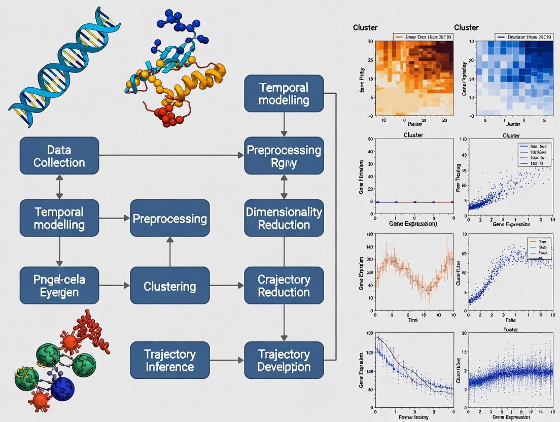
The following diagram illustrates the conceptual framework and workflow for reconstructing cellular dynamics from snapshot data:

The diagram above illustrates how different computational approaches extract temporal information from static snapshots to reconstruct dynamic trajectories, ultimately leading to insights into biological mechanisms.

The Scientist's Toolkit: Essential Research Reagents and Computational Tools

Table 2: Essential Research Reagents and Computational Tools for Dynamic Single-Cell Analysis

Tool/Reagent	Type	Function	Application Context
scRNA-seq Platforms (10X Genomics, Smart-seq2)	Experimental Platform	High-throughput gene expression profiling at single-cell resolution	Generating input snapshot data for all dynamic inference methods
RNA Metabolic Labeling (SLAM-seq, scNT-seq)	Experimental Method	Tags newly synthesized RNA for direct measurement of transcription kinetics	Ground truth for RNA velocity parameter estimation; studying transcriptional bursts
Lineage Tracing (CRISPR-based recording)	Experimental Method	Records ancestral relationships between cells using DNA barcodes	Constraining trajectory inference with clonal relationship information
Spatial Transcriptomics (MERFISH, seqFISH)	Experimental Method	Preserves spatial context during transcriptome profiling	Integrating spatial organization with temporal dynamics
TDEseq	Computational Tool	Detects temporal expression patterns using spline-based mixed models	Identifying genes with specific dynamic patterns across multiple time points
TIGON	Computational Tool	Reconstructs trajectories with growth using unbalanced optimal transport	Modeling developmental processes with cell population changes
scVelo	Computational Tool	Infers RNA velocity using dynamical modeling	Predicting short-term future cell states from splicing kinetics
CellRank	Computational Tool	Models state transitions using RNA velocity and graph neural networks	Identifying transition probabilities between cell states
Fen1-IN-5	Fen1-IN-5, MF:C21H17N3O4S, MW:407.4 g/mol	Chemical Reagent	Bench Chemicals
5-Morpholin-4-yl-8-nitro-quinoline	5-Morpholin-4-yl-8-nitro-quinoline	5-Morpholin-4-yl-8-nitro-quinoline is a quinoline derivative for research use only (RUO). Explore its applications in developing novel therapeutic agents. Not for human consumption.	Bench Chemicals

Future Perspectives: Toward a Truly Dynamic Single-Cell Biology

The field of temporal modeling in single-cell transcriptomics is rapidly evolving, with several emerging directions poised to address current limitations. Live-cell transcriptomics methods, such as Live-seq, enable transcriptomic profiling without cell destruction, providing an assumption-free measurement of dynamics [4]. This approach utilizes fluidic force microscopy (FluidFM) to extract cytoplasmic biopsies while preserving cell viability, allowing direct longitudinal monitoring of the same cells over time [4].

The integration of multimodal measurements—combining transcriptomics with epigenomics, proteomics, and spatial information—represents another promising frontier [2]. As the scale of single-cell datasets continues to grow, with experiments now profiling millions of cells, new computational approaches must address challenges in scaling to higher dimensionalities while quantifying uncertainty of measurements and analysis results [2]. Future methods will likely combine the strengths of computational inference with direct temporal measurements through innovative experimental designs, ultimately providing a more complete understanding of cellular dynamics in development, disease, and therapeutic interventions.

For researchers and drug development professionals, these advances offer the potential to move beyond descriptive cellular taxonomies to predictive models of cell fate decisions, enabling more targeted therapeutic interventions that account for the dynamic nature of cellular responses in complex biological systems.

Single-cell RNA sequencing (scRNA-seq) has revolutionized biology by enabling high-throughput quantification of gene expression at individual cell resolution, allowing researchers to investigate cellular heterogeneity at unprecedented resolution. However, a fundamental challenge persists: standard scRNA-seq provides only static cellular snapshots of gene expression, obscuring dynamic temporal processes such as differentiation, reprogramming, and disease progression [8] [3]. During development and homeostasis, cells undergo continuous transitions, adapting their transcriptional programs to coordinate behavior. To reconstruct these dynamic processes from static snapshots, computational biologists have developed three principal classes of temporal inference methods: pseudotime analysis, RNA velocity, and trajectory inference [8] [9].

These methods computationally order cells along developmental trajectories, allowing the unbiased study of cellular dynamic processes. The overarching goal is to map the developmental or disease history of differentiated cells, a fundamental objective in developmental and stem cell biology with significant impacts for regenerative medicine and cancer biology [8]. Since 2014, more than 70 trajectory inference tools have been developed, creating both opportunities and challenges for researchers seeking to apply these methods [10] [11]. This article provides a comprehensive overview of the core concepts, methodological comparisons, experimental protocols, and recent advances in pseudotime analysis, RNA velocity, and cell trajectory inference, framed within the broader context of temporal modelling in single-cell transcriptomics research.

Core Concepts and Methodological Foundations

Pseudotime Analysis

Pseudotime analysis refers to computational approaches that order individual cells along a hypothetical temporal trajectory based on their transcriptional similarities [8] [12]. The fundamental assumption is that cells with similar gene expression profiles are likely at similar stages of a developmental process. Pseudotime algorithms take a collection of cell states represented in a high-dimensional space and identify a one-dimensional, latent representation of cellular states that corresponds to developmental progression [8].

The technical workflow typically begins with a researcher defining a starting cell population (e.g., progenitor or stem cells) based on prior knowledge of the experimental system [8]. The algorithm then orders the cell state manifold by calculating the transcriptional distance of each cell from this starting point, assigning a pseudotime value to each cell representing its relative progression along the trajectory [8]. Mathematically, pseudotime is defined as the distance along a smooth continuous curve that passes through the cell state manifold, representing the most likely trajectory of cell transitions [8].

A key limitation of pseudotime approaches is their dependence on prior knowledge for setting the starting point, which can introduce bias if this knowledge is inaccurate or incomplete [8]. Additionally, these methods assume that transcriptional similarity directly implies developmental relationships, which may not always hold true [8]. For example, in early mammalian development, primitive and definitive endoderm have similar expression profiles but emerge from different precursors at different developmental stages [8].

RNA Velocity

RNA velocity is a groundbreaking computational method that predicts the future transcriptional state of individual cells by leveraging the ratio of unspliced (pre-mRNA) to spliced (mature mRNA) transcripts [8] [3]. The method is based on the fundamental observation that the timescale of cellular development is comparable to the kinetics of the mRNA life cycle: transcription of precursor mRNA, splicing to produce mature mRNA, followed by mRNA degradation [8].

The core principle states that if the ratio of unspliced to spliced mRNA is in balance, this indicates homeostasis (steady state), while an imbalance indicates future induction or repression in gene expression [8]. By comparing these ratios for each gene across cells, RNA velocity can infer both the direction and speed of gene expression changes along developmental trajectories [8]. This allows researchers to predict differentiation potential, identify fate decisions, and discover key regulators of cell transitions [8].

RNA velocity adds a temporal dimension to single-cell transcriptomics and can improve the accuracy and resolution of trajectory inference. The velocity vectors obtained for each cell can be projected into low-dimensional embeddings (e.g., UMAP or t-SNE) to visualize the directional flow of cells [8]. However, the method relies on several assumptions, including constant, gene-specific splicing rates that may not hold true in all biological contexts, and requires substantial cell numbers and sequencing depth for reliable estimates [8].

Trajectory Inference Methods

Trajectory inference approaches represent a broader class of methods that analyze genome-wide omics data from thousands of single cells to computationally infer the order of these cells along developmental trajectories [10]. These methods aim to reconstruct the underlying cellular dynamics from static snapshots, essentially connecting discrete cell states into continuous processes [9].

The initial methodological development focused on adapting approaches based on clustering or graph traversal, but recent advances have extended the field in multiple directions [9]. Current methods include probabilistic approaches that report uncertainties about their outputs, and methods that incorporate complementary knowledge such as unspliced mRNA, time point information, or other omics data to construct more accurate trajectories [9]. The trajectory models can take various topologies including linear, bifurcating, multifurcating, cyclic, or tree-like structures, reflecting the complexity of biological processes [10].

Table 1: Comparison of Major Temporal Inference Approaches

Method Type	Core Data Input	Underlying Principle	Key Advantages	Major Limitations
Pseudotime Analysis	Spliced mRNA counts	Transcriptional similarity from a defined start point	Intuitive ordering; Multiple algorithms available	Requires prior knowledge for start point; Assumes transcriptional similarity reflects developmental relationship
RNA Velocity	Both unspliced and spliced mRNA counts	mRNA splicing kinetics	Predicts future states; Does not require start point	Assumes constant splicing rates; Requires high sequencing depth
Trajectory Inference	Typically spliced mRNA counts	Graph traversal or probabilistic modeling	Can capture complex topologies; Comprehensive benchmarking available	Model misspecification; Varying performance across topology types

Comparative Performance and Benchmarking

As the number of trajectory inference methods has grown exponentially, comprehensive benchmarking studies have become essential for guiding methodological selection. A landmark 2019 study in Nature Biotechnology evaluated 45 trajectory inference methods on 110 real and 229 synthetic datasets, assessing performance across multiple metrics including cellular ordering accuracy, network topology correctness, scalability, and usability [10].

The results highlighted the complementarity of existing tools, demonstrating that method performance depends significantly on dataset dimensions and trajectory topology [10]. Some methods, including Slingshot, TSCAN, and Monocle DDRTree, consistently outperformed others in specific trajectory types [10] [12]. The benchmarking analysis indicated that while current methods perform well on simple trajectories, there remains considerable room for improvement, particularly for detecting complex trajectory topologies [10] [12].

This benchmarking effort led to the development of practical guidelines to help researchers select appropriate methods for their specific datasets, available through the dynverse platform [10]. The evaluation pipeline and data remain freely available, supporting continued development of improved tools designed to analyze increasingly large and complex single-cell datasets [10].

Table 2: Performance of Selected Trajectory Inference Methods Across Different Topologies

Method Name	Linear Trajectories	Bifurcating Trajectories	Multifurcating Trajectories	Cyclic Trajectories	Tree-like Trajectories
Slingshot	High accuracy	High accuracy	Moderate accuracy	Not applicable	Low accuracy
TSCAN	High accuracy	Moderate accuracy	Low accuracy	Moderate accuracy	Low accuracy
Monocle DDRTree	High accuracy	High accuracy	High accuracy	Not applicable	Moderate accuracy
PAGA	Moderate accuracy	High accuracy	High accuracy	Low accuracy	High accuracy
SCORPIUS	High accuracy	Moderate accuracy	Low accuracy	Not applicable	Low accuracy

Experimental Protocols and Workflows

Standard Protocol for RNA Velocity Analysis

A robust protocol for RNA velocity analysis involves multiple stages from experimental design to computational interpretation:

Sample Preparation and Sequencing

• Isolate cells of interest using standard single-cell protocols (FACS, microfluidics, etc.)
• Prepare libraries using scRNA-seq protocols that preserve intronic reads (e.g., 10X Genomics, inDrops)
• Sequence with sufficient depth to capture both spliced and unspliced transcripts (typically >50,000 reads/cell)

Data Preprocessing

• Quality control: Filter cells with low RNA content, high mitochondrial percentage, or outlier gene counts
• Preprocessing: The unspliced and spliced RNA abundances are preprocessed for velocity gene selection and pseudotime initialization [13]
• Dimensionality reduction: Perform PCA, UMAP, or t-SNE to project data into lower-dimensional space

Velocity Estimation

• Employ tools like Velocyto, scVelo, or Dynamo to estimate RNA velocity
• For in situ RNA velocity analysis, nuclear and cytoplasmic mRNA counts can substitute for unspliced and spliced counts [14]
• Visualize velocity vectors projected onto embedding (UMAP/t-SNE) to assess directionality

Trajectory Inference

• Apply trajectory inference methods (Slingshot, PAGA, Monocle) to reconstruct developmental paths
• Validate trajectories using known marker genes and developmental biology knowledge

Downstream Analysis

• Identify key regulator genes along trajectories
• Construct dynamic gene regulatory networks
• Perform differential expression testing across pseudotime

Advanced Protocol: TIGON for Dynamic Trajectory Inference

TIGON represents a recent advanced methodology that uses dynamic, unbalanced optimal transport to reconstruct dynamic trajectories and population growth simultaneously from multiple snapshots [15]. The protocol involves:

Input Data Preparation

• Collect time-series scRNA-seq data at multiple time points
• Estimate density functions at discrete time points using Gaussian mixture models
• Perform dimension reduction (PCA, UMAP, or autoencoder) to project into lower-dimensional space

Model Implementation

• Implement Wasserstein-Fisher-Rao (WFR) distance minimization using neural ODEs
• Approximate velocity v(x,t) and growth g(x,t) using neural networks
• Solve the hyperbolic partial differential equation: ∂tρ(x,t) + ∇·(v(x,t)ρ(x,t)) = g(x,t)ρ(x,t)

Trajectory and Growth Reconstruction

• Track cell dynamics by integrating along the velocity field
• Assess gene contributions to growth from the gradient of growth (∇g)
• Construct gene regulatory networks from the Jacobian of velocity

Validation

• Compare inferred trajectories with known lineage tracing data
• Validate growth predictions using experimental growth measurements
• Assess regulatory networks using known transcription factor-target relationships

Diagram 1: Single-cell trajectory analysis workflow

Recent Methodological Advances

Integration of Multi-Omics Data

Recent trajectory inference methods increasingly incorporate multi-omics data to enhance accuracy and biological relevance. Methods like MultiVelo extend RNA velocity analysis to single-cell ATAC-seq datasets, while protaccel extends it to protein abundance [13]. These integrated approaches recognize that cellular identity and fate decisions are determined through complex interactions between transcriptional, epigenetic, and proteomic layers.

TIGON represents another significant advancement by simultaneously modeling cell velocity and population growth within a unified optimal transport framework [15]. Traditional methods often assume constant cell numbers or neglect proliferation and death effects, potentially misrepresenting true dynamics. TIGON's incorporation of growth terms addresses this limitation, particularly important in developmental contexts with rapid cell division [15].

Deep Learning Approaches

Neural ordinary differential equations (ODEs) have emerged as powerful tools for modeling single-cell dynamics. TSvelo exemplifies this approach, implementing a comprehensive RNA velocity framework that models the cascade of gene regulation, transcription, and splicing using interpretable neural ODEs [13]. Unlike methods that treat genes independently, TSvelo integrates transcriptional regulation information from TF-target databases while maintaining parameter interpretability [13].

Another innovation involves generative models such as VeloVI, veloVAE, and Pyrovelocity, which utilize Bayesian frameworks to estimate RNA velocity with uncertainty quantification [13]. These approaches better account for the sparsity and noise inherent in single-cell data, particularly for genes with low expression levels.

Spatial Trajectory Inference

The integration of spatial information with trajectory inference represents a frontier in single-cell analytics. Methods like STT and SIRV extend RNA velocity analysis to spatial transcriptomics, enabling researchers to reconstruct developmental trajectories while preserving tissue architecture context [13]. For imaging-based spatial transcriptomics methods like MERFISH, RNA velocity can be inferred by distinguishing between nuclear and cytoplasmic mRNAs rather than spliced/unspliced ratios [14].

Diagram 2: Evolution of trajectory inference concepts

Successful implementation of pseudotime, RNA velocity, and trajectory analysis requires both wet-lab reagents and computational resources. Below are essential components for designing experiments in this domain:

Table 3: Essential Research Reagents and Computational Tools

Resource Type	Specific Examples	Primary Function	Key Considerations
Single-cell RNA-seq Platforms	10X Genomics, inDrops, SMART-seq2	Generate single-cell transcriptome data	Protocol choice affects detection of unspliced transcripts
Spatial Transcriptomics Platforms	MERFISH, Seq-Scope, 10X Visium	Provide spatial context for gene expression	Compatibility with RNA velocity analysis varies
Lineage Tracing Systems	CRISPR-based barcoding, fluorescent reporters	Establish ground truth for lineage relationships	May require custom computational integration
Reference Databases	ChEA, ENCODE TF-target databases	Provide prior knowledge for regulatory inference	Database selection influences regulatory network predictions
Velocity Estimation Tools	Velocyto, scVelo, Dynamo, TSvelo	Calculate RNA velocity from spliced/unspliced counts	Underlying assumptions and model complexity vary
Trajectory Inference Software	Slingshot, Monocle, PAGA, TSCAN	Reconstruct developmental trajectories from single-cell data	Performance depends on trajectory topology
Benchmarking Platforms	dynverse, BEELINE	Compare method performance and select optimal approaches	Essential for rigorous methodological selection
Visualization Tools	scVelo, Scanpy, Seurat	Project trajectories and velocities onto low-dimensional embeddings	Critical for biological interpretation and communication

The field of temporal modeling in single-cell transcriptomics has evolved dramatically from initial pseudotime approaches to increasingly sophisticated methods that integrate multiple data modalities and leverage advanced computational frameworks. Current methods like TIGON and TSvelo demonstrate the power of combining optimal transport theory with neural ODEs to reconstruct complex developmental trajectories while accounting for population growth and gene regulatory networks [15] [13].

Looking forward, several challenges and opportunities remain. There is a growing need for methods that can better handle complex trajectory topologies, including loops, alternative paths, and cross-differentiation events [8] [10]. The integration of single-cell multi-omics data—including epigenomic, proteomic, and spatial information—will continue to enhance trajectory inference accuracy [9] [13]. Additionally, approaches that provide uncertainty quantification and robust statistical frameworks will be essential for translating trajectory inferences into biologically meaningful insights, particularly for clinical applications [9] [3].

For researchers and drug development professionals, these advances in temporal modeling offer unprecedented opportunities to map disease progression, identify novel therapeutic targets, and understand drug mechanisms at cellular resolution. As the field continues to mature, we anticipate that trajectory inference methods will become increasingly integral to both basic biological discovery and translational applications across diverse domains including developmental biology, cancer research, and regenerative medicine.

Single-cell RNA sequencing (scRNA-seq) has revolutionized our ability to characterize cellular heterogeneity, but traditional approaches present a fundamental limitation: they require cell lysis, providing only a single snapshot in time and impeding further molecular or functional analyses on the same cells [16] [17]. This destructive sampling creates a critical challenge in understanding how a cell's molecular state influences its response to perturbations, such as inflammatory signals or differentiation stimuli [16]. To address this, the field has developed innovative experimental designs that incorporate a temporal dimension, broadly categorized into computational inference methods and experimental recording techniques. Computational approaches like pseudotime ordering infer continuous trajectories based on transcriptome similarity, while experimental methods such as Live-seq directly record temporal changes by preserving cell viability [17]. This article details these methodologies, their protocols, and applications, providing a comprehensive toolkit for researchers investigating dynamic biological processes.

The table below summarizes the core experimental designs for capturing temporal information in single-cell transcriptomics, highlighting their fundamental principles, outputs, and key considerations.

Table 1: Strategies for Capturing Temporal Dynamics in Single-Cell Transcriptomics

Strategy	Core Principle	Temporal Output	Key Advantage	Primary Limitation
Live-seq [16] [18]	Cytoplasmic biopsy via FluidFM to extract mRNA while preserving cell viability.	Direct, sequential transcriptome measurements from the same live cell.	Enables direct coupling of a cell's ground state to its downstream phenotypic behavior.	Lower RNA recovery leading to fewer genes detected per cell compared to scRNA-seq.
Time-Series scRNA-seq [19]	Destructive sampling of cells from the same population at multiple time points.	A series of population-level snapshots across different time points.	Technically straightforward; uses established scRNA-seq protocols.	Cannot track the same cell over time; relies on population-level inference.
Time-Resolved Reporters [20]	Genetically engineered reporter systems (e.g., Gcg-Timer) that label cells based on their activation or differentiation state.	Indirect temporal information by distinguishing early vs. late cell states within a single sample.	Provides high temporal resolution for specific cell lineages without complex computations.	Limited to predefined biological processes and requires genetic modification.
Computational Inference (e.g., Pseudotime) [21] [17]	Algorithmic ordering of single-cell snapshots along a reconstructed trajectory based on transcriptome similarity.	Inferred continuous trajectory representing a biological process (e.g., development).	Can be applied to existing scRNA-seq data; no specialized wet-lab protocols needed.	Result is a statistical inference, not an actual timeline; directionality can be ambiguous.

Detailed Experimental Protocols

Protocol 1: Live-seq for Temporal Transcriptomic Recording

Live-seq transforms scRNA-seq from an end-point to a temporal analysis approach by using fluidic force microscopy (FluidFM) to perform cytoplasmic biopsies, allowing sequential molecular profiling of the same cell [16] [18].

Workflow Diagram: Live-seq

Step-by-Step Methodology:

• Probe Preparation: Preload a FluidFM probe (with an aperture of 300-500 nm) with a sampling buffer containing RNase inhibitors. This is critical to immediately stabilize the minimal amount of RNA upon extraction [16].
• Cell Selection and Biopsy: Place the cell culture dish on the stage of an inverted microscope integrated with the FluidFM system. Use image-based cell tracking to identify and position a target cell. Lower the probe onto the cell membrane, apply gentle force and suction to penetrate the membrane and extract approximately 1 picoliter of cytoplasm [16].
• Sample Collection: Retract the probe and release the cytoplasmic extract into a microliter-scale droplet containing a buffer compatible with downstream RNA-seq library construction. Implement a stringent wash protocol for the FluidFM probe (>99% accuracy) between cells to prevent cross-contamination [16].
• Low-Input RNA Sequencing: Convert the extracted mRNA into a sequencing library using an optimized, high-sensitivity version of the Smart-seq2 protocol. This enhanced workflow is capable of reliably detecting as little as 1 picogram of total RNA, a necessity given the minimal input material [16].
• Downstream Phenotypic Monitoring: Following biopsy, the cell remains viable in culture. It can be subjected to various perturbations (e.g., LPS stimulation, differentiation induction) and monitored over time via time-lapse imaging or other functional assays to link its initial transcriptomic state to its subsequent behavior [16] [18].

Protocol 2: Time-Series scRNA-seq with Computational Trajectory Modeling

This design involves sacrificially harvesting cells from a population at multiple time points during a dynamic process, followed by scRNA-seq and computational analysis to reconstruct temporal trajectories [19].

Workflow Diagram: Time-Series scRNA-seq Analysis

Step-by-Step Methodology:

• Experimental Time-Series Design: Plan and execute the biological experiment, collecting cells from the population at key time points. For example, collect immune cells before and at several intervals after stimulation, or collect cells at different stages of embryonic development [20] [19].
• Single-Cell Library Preparation and Sequencing: For each time point, prepare a single-cell suspension. Generate barcoded scRNA-seq libraries using a preferred platform (e.g., droplet-based 10x Genomics, or full-length Smart-seq2 for higher sensitivity). Pool and sequence the libraries [22] [23].
• Data Preprocessing and Integration: Process the raw sequencing data to generate a gene expression count matrix for each cell. Use tools like Seurat or Scanpy to perform quality control, normalize data, and integrate cells from different time points to correct for batch effects [23].
• Trajectory Inference: Apply pseudotime inference algorithms such as Slingshot [21], Monocle, or TSCAN. These tools order individual cells along a reconstructed trajectory based on transcriptomic similarity, effectively creating a "pseudotime" axis from the start to the end of the biological process [21] [17] [19].
• Analysis of Dynamic Gene Behavior: Model how gene expression and interactions change along the inferred pseudotime.
  • Differential Expression: Use tools like tradeSeq to identify genes with non-linear expression changes over pseudotime [21].
  • Gene Co-Expression Analysis: Employ methods like TIME-CoExpress, a copula-based framework that models non-linear changes in gene-gene co-expression patterns, dynamic zero-inflation rates, and mean expression levels along the temporal trajectory [21].

The Scientist's Toolkit: Key Research Reagent Solutions

Successful implementation of temporal single-cell transcriptomics relies on a suite of specialized reagents and platforms. The table below catalogues essential solutions for key methodological steps.

Table 2: Essential Research Reagent Solutions for Temporal scRNA-seq

Category / Reagent	Specific Examples	Function & Application Note
Library Prep Kits
- High-Sensitivity Full-Length	Smart-seq2, Smart-seq3 [17]	Optimal for Live-seq and low-input samples; provides full transcript coverage. Smart-seq3 offers improved sensitivity with 5'-UMI counting.
- High-Throughput 3'	10x Genomics Chromium, Parse Biosciences Evercode [22] [24]	For large time-series studies. Parse's combinatorial barcoding can process millions of cells from thousands of samples.
Cell Capture & Isolation
- Microfluidics Platform	10x Genomics, BD Rhapsody [22] [23]	Encapsulates single cells into droplets or microwells for barcoding.
- Fluorescence-Activated Cell Sorting (FACS)	N/A [23]	Enriches for specific cell populations prior to sequencing (e.g., using fluorescent reporters like Gcg-Timer [20]).
Critical Enzymes & Buffers
- Reverse Transcriptase	Superscript IV (SSRTIV) [17]	Used in FLASH-seq for higher processivity, improving gene detection in full-length protocols.
- RNase Inhibitors	N/A [16]	Essential for Live-seq to preserve RNA integrity during and after cytoplasmic extraction.
Specialized Systems
- Fluidic Force Microscopy	FluidFM [16] [18]	The core technology enabling Live-seq, allowing for cytoplasmic extraction with minimal invasiveness.
CCK-A receptor inhibitor 1	CCK-A receptor inhibitor 1, MF:C25H35NO6S, MW:477.6 g/mol	Chemical Reagent
Z-Arg-SBzl	Z-Arg-SBzl, MF:C21H26N4O3S, MW:414.5 g/mol	Chemical Reagent

Application Notes in Biological Research

Immune Response and Macrophage Polarization

Live-seq has been applied to pre-register the transcriptomes of individual macrophages before stimulating them with lipopolysaccharide (LPS). This enabled the identification of basal gene expression features, such as Nfkbia levels and cell cycle state, which predicted the strength of the subsequent inflammatory response, uncovering determinants of response heterogeneity [16].

Pancreatic Cell Development and Differentiation

Time-resolved reporter systems, such as the Gcg-Timer mouse, allow for the isolation of early versus late α-cells during embryonic development at E17.5. scRNA-seq of these sorted populations revealed transcriptional dynamics, showing that early α-cells express key β-cell genes like Ins1 and Ins2 before maturing into Gcg-high late α-cells, providing insights into endocrine cell differentiation [20].

Drug Discovery and Biomarker Identification

In drug development, time-series scRNA-seq can profile cellular responses to compounds at multiple doses and time points. This identifies cell-type-specific transcriptomic changes, mechanisms of efficacy and resistance, and predictive biomarkers. The ability to stratify patients based on dynamic molecular responses within cell subpopulations is invaluable for personalized medicine [24].

The integration of temporal resolution into single-cell transcriptomics is rapidly advancing our understanding of dynamic biological systems. Experimental designs now range from repeated destructive sampling to the groundbreaking Live-seq technology, which allows direct longitudinal tracking of the same cell. Coupled with sophisticated computational models for analyzing time-series and pseudotime data, these methods provide a powerful means to move beyond static snapshots. As these protocols continue to mature—driving increases in sensitivity, throughput, and analytical depth—they will undoubtedly unlock deeper insights into developmental biology, disease progression, and therapeutic interventions, firmly establishing time as a fundamental dimension in single-cell research.

Key Biological Questions Addressed by Temporal Modeling (e.g., Differentiation, Immune Response)

Biological systems are inherently dynamic, with processes such as cellular differentiation, immune response, and disease progression unfolding over time. Single-cell RNA sequencing (scRNA-seq) has revolutionized our ability to observe these processes by providing high-resolution views of transcriptomic states at the cellular level. However, conventional scRNA-seq offers only static snapshots, posing significant challenges for understanding temporal sequences and causal relationships [25].

Temporal modeling computational frameworks bridge this gap by ordering cells along pseudotime trajectories, inferring RNA velocity, and integrating multi-omics data to reconstruct dynamic biological pathways. These approaches have become indispensable for addressing fundamental biological questions that involve state transitions and temporal progression [26]. This article explores the key biological questions where temporal modeling provides critical insights, detailing the experimental and computational protocols that enable these discoveries.

Key Biological Questions and Applications

Temporal modeling of single-cell transcriptomic data has been successfully applied to address several fundamental questions in biology and medicine. The table below summarizes the primary biological questions, key findings, and analytical techniques used in recent studies.

Table 1: Key Biological Questions Addressed by Temporal Modeling

Biological Question	Key Findings	Analytical Techniques	References
Cellular Differentiation & Development	Ordered lineage commitment, temporal specificity of disorder-risk genes in brain development, pituitary gland embryogenesis	Pseudotime analysis, RNA velocity, trajectory inference, gene co-expression dynamics	[21] [27]
Immune Response Dynamics	Rapid activation of intestinal CD8+ T cells and plasma cells during Salmonella infection; "immune clock" in sepsis with defined critical windows	scIVNL-seq for new/old RNA, differential equation models, multi-omics fusion	[28] [29]
Disease Progression	Transition from ductal carcinoma in situ (DCIS) to invasive ductal carcinoma (IDC) in breast cancer; identification of T cell subsets and key prognostic genes	Cell-cell communication analysis, pseudotime trajectory of T cells, WGCNA	[30]
Therapeutic Intervention Timing	Identification of two intervention windows in sepsis (0-18h and 36-48h) forecasting 2.1-fold and 1.6-fold survival gains, respectively	Dynamic simulations, ordinary differential equations (ODEs), stochastic differential equations (SDEs)	[29]

Experimental Protocols for Temporal Resolution

Metabolic Labelling for RNA Dynamics

Protocol: scIVNL-seq (Single-cell In Vivo New RNA Labeling Sequencing)

Purpose: To distinguish newly synthesized transcripts from pre-existing RNAs, providing direct measurement of transcriptional activity and degradation in vivo [28].

Workflow Diagram:

Key Reagents and Solutions:

• 4-thiouridine (S4U): Nucleoside analog incorporated into nascent RNA during transcription [28] [26].
• Tail Vein Catheterization Setup: For precise intravenous administration in mouse models.
• Cell Dissociation Kit: Tissue-specific enzymatic mix for single-cell suspension preparation.
• 10x Genomics Chromium System: For droplet-based single-cell encapsulation and barcoding.
• UMI (Unique Molecular Identifier) Adapters: For digital counting and accurate transcript quantification.

Multi-Omics Integration for Temporal Networks

Protocol: Multi-Omics Temporal Network Reconstruction in Sepsis

Purpose: To integrate scRNA-seq, ATAC-seq, and CITE-seq data for reconstructing a time-resolved "immune clock" of sepsis progression, identifying critical checkpoints and intervention windows [29].

Workflow Diagram:

Key Reagents and Solutions:

• Cell Hashing Antibodies: For sample multiplexing and demultiplexing in CITE-seq.
• Tn5 Transposase: For tagmentation in ATAC-seq library preparation.
• Feature Barcoding Kit: For simultaneous surface protein detection.
• scMGNN Tool: Computational tool for multi-omics data harmonization [29].
• Palantir: For pseudotime analysis and trajectory construction [27].

Computational Methods for Temporal Modeling

Pseudotime and Trajectory Inference

Protocol: TIME-CoExpress for Dynamic Co-Expression Analysis

Purpose: To model non-linear changes in gene co-expression patterns, zero-inflation rates, and mean expression levels along cellular temporal trajectories [21].

Table 2: Comparison of Computational Methods for Temporal Modeling

Method	Primary Function	Key Features	Limitations
TIME-CoExpress	Models non-linear gene co-expression	Copula-based framework, handles zero-inflation, multi-group comparison	Computationally intensive for large gene sets [21]
Slingshot	Pseudotime inference	Unsupervised, robust to noise, multiple lineage inference	Requires predefined clusters [21]
Monocle	Pseudotime and trajectory analysis	Orders cells using transcriptome similarity	Infers rather than measures true time [26]
RNA Velocity	Predicts future cell states	Based on spliced/unspliced RNA ratio	More applicable to steady-state models [26]
scHOT	Detects changing gene interactions	Uses Spearman's correlation along trajectories	Cannot simultaneously analyze multiple groups [21]

Workflow Diagram:

Signaling Pathway Dynamics Visualization

Protocol: Temporal Analysis of Immune Signaling Pathways

Application: Mapping the dynamics of critical signaling pathways (e.g., NF-κB, PD-1/TIM-3) during immune activation and exhaustion in sepsis and cancer [29] [30].

Workflow Diagram:

The Scientist's Toolkit

Table 3: Essential Research Reagent Solutions for Temporal scRNA-seq Studies

Category	Item	Function	Example Applications
Metabolic Labeling	4-thiouridine (S4U)	Labels nascent RNA for transcriptional dynamics	scIVNL-seq, scSLAM-seq [28] [26]
Metabolic Labeling	TimeLapse Chemistry	Converts S4U to cytosine analogue for droplet-based platforms	scNT-seq [25]
Cell Sorting	Fluorescent Reporters (e.g., Neurog3Chrono)	Visualizes temporal progression via fluorescent protein ratios	Cell fate tracing studies [25]
Single-Cell Profiling	10x Genomics Chromium	High-throughput single-cell encapsulation and barcoding	Most large-scale scRNA-seq studies [30]
Multi-Omics	CITE-seq Antibodies	Simultaneous measurement of surface proteins	Immune cell phenotyping [29]
Multi-Omics	ATAC-seq Reagents	Chromatin accessibility profiling	Regulatory network inference [29]
Computational Tools	scVILNL-seq Analysis Pipeline	Quantifies new vs. old RNA and calculates transcription rates	Immune response studies [28]
Computational Tools	TIME-CoExpress R/Package	Identifies dynamic gene co-expression patterns	Developmental studies [21]
Fotagliptin	Fotagliptin, MF:C17H19FN6O, MW:342.4 g/mol	Chemical Reagent	Bench Chemicals
N-(4-acetylphenyl)sulfonylacetamide	N-(4-Acetylphenyl)sulfonylacetamide|Research Chemical	High-purity N-(4-Acetylphenyl)sulfonylacetamide for research applications. This product is for laboratory research use only and not for human consumption.	Bench Chemicals

The Computational Toolbox: Methods for Inferring and Modeling Cellular Trajectories

Trajectory Inference and Pseudotime Ordering with Tools like Slingshot and Monocle

Single-cell RNA sequencing (scRNA-seq) has revolutionized biology by allowing researchers to profile transcript abundance at the resolution of individual cells, opening new avenues to study dynamic processes such as cell differentiation, development, and disease progression [31] [32]. However, standard scRNA-seq provides only static cellular snapshots, obscuring temporal processes because the technique is inherently destructive to cells [31] [33]. Trajectory inference (TI) has emerged as a powerful computational approach to overcome this limitation by ordering cells along inferred developmental trajectories based on transcriptional similarities [31]. This ordering produces a "pseudotime" value for each cell, representing its relative progression along a continuous biological process [34]. For example, in differentiation processes, pseudotime can represent the degree of differentiation from a pluripotent stem cell to a fully differentiated terminal state [34].

The core assumption underlying trajectory inference is that cells undergoing transitions between states will create a continuum in gene expression space, and that sufficient sampling will capture cells at various points along these transitions [31]. TI methods aim to connect these cells through their transcriptional similarities, effectively reconstructing the temporal dynamics from static snapshots [31] [32]. These approaches have become indispensable for studying processes where direct temporal monitoring is impossible, allowing researchers to map complex lineage relationships and identify molecular drivers of cellular fate decisions [31] [32]. Within the broader context of temporal modelling in single-cell transcriptomics development research, trajectory inference provides a foundational framework for understanding how gene expression programs unfold over time, offering insights into normal development, disease mechanisms, and potential therapeutic interventions [3].

Theoretical Foundations of Pseudotime and Lineage Inference

Conceptual Framework of Pseudotime

Pseudotime is a computational construct that quantifies the relative progression of individual cells along a biological process [34]. It is important to note that "pseudotime" may not have a linear relationship with real chronological time; rather, it represents transcriptional progression along a continuum [34]. For time-dependent processes like differentiation, pseudotime can serve as a proxy for relative cellular age, but only when directionality can be reliably inferred [34]. In branched trajectories, cells typically receive multiple pseudotime values—one for each path through the trajectory—and these values are generally not comparable across different paths [34].

The mathematical inference of pseudotime relies on the assumption that cells with similar transcriptional profiles occupy similar positions in the developmental continuum [31]. The process begins with dimensionality reduction to address the high-dimensional nature of scRNA-seq data, followed by the inference of global lineage structures, and finally the projection of cells onto these structures to assign pseudotime values [32]. A critical consideration is whether a continuous trajectory actually exists in the dataset, as continua can sometimes be interpreted as series of closely related but distinct subpopulations, while separated clusters might represent endpoints of a trajectory with rare intermediates [34]. This interpretive flexibility requires analysts to choose perspectives based on biological plausibility and utility [34].

Methodological Approaches to Lineage Inference

Multiple computational approaches have been developed for lineage inference, each with distinct theoretical foundations and algorithmic strategies. Cluster-based minimum spanning tree (MST) methods, implemented in tools like TSCAN and the first stage of Slingshot, cluster cells then construct a minimum spanning tree on cluster centroids to identify the most parsimonious connections between cellular states [34] [33]. The MST provides an intuitive representation of transitions between clusters, with paths through the tree representing potential lineages [34]. Principal curves approaches, used in the second stage of Slingshot and similar methods, fit smooth one-dimensional curves that pass through the middle of data in high-dimensional space, providing a nonlinear summary of the data [35] [33]. These curves effectively capture continuous transitions without discrete clustering steps. Graph-based learning methods, employed by Monocle 2 and later versions, use machine learning strategies like reversed graph embedding to learn principal graphs that describe the single-cell dataset while simultaneously mapping points back to the original high-dimensional space [33]. Partition-based graph abstraction, implemented in PAGA, creates graph representations of cellular relationships using a multi-resolution approach that combines clustering and continuous transition models [31].

Each approach presents distinct advantages: cluster-based methods offer computational efficiency and noise resistance [34]; principal curves provide smooth, continuous representations [35]; graph-learning methods capture complex branching patterns [33]; and partition-based approaches handle disconnected clusters and sparse sampling effectively [31]. The choice among these methodologies depends on dataset characteristics, trajectory complexity, and analytical goals.

Comparative Analysis of Slingshot and Monocle

Slingshot represents a modular approach to trajectory inference that combines cluster-based stability with flexible curve-fitting [35]. Its algorithm consists of two distinct stages: first, it identifies global lineage structure using a cluster-based minimum spanning tree (MST), which stably identifies the number of lineages and branching points; second, it fits simultaneous principal curves to these lineages to estimate cell-level pseudotime variables for each lineage [35] [33]. This two-stage approach provides robustness to noise—a critical feature for noisy single-cell data—while accommodating multiple branching lineages [35]. A key advantage of Slingshot is its flexibility regarding upstream preprocessing steps; it does not require specific clustering, normalization, or dimensionality reduction methods, allowing integration into diverse analytical workflows [35].

Monocle exists in several iterations, each with distinct algorithmic approaches. The original Monocle constructed a minimum spanning tree on individual cells using independent component analysis (ICA) and ordered cells via a PQ tree along the longest path [35]. Monocle 2 introduced reversed graph embedding (RGE), specifically using DDRTree (Discriminative Dimensionality Reduction via Learning a Tree), to simultaneously learn a principal graph and map cells onto it [33]. Monocle 3 further evolved this approach by using UMAP for dimensionality reduction, Louvain/Leiden algorithms for clustering, and a variant of SimplePPT algorithm to construct trajectories that can accommodate multiple origins, cycles, and converging states [31] [33]. Unlike Slingshot's two-stage process, Monocle 3 integrates dimensionality reduction, clustering, and graph construction into a more unified framework.

Performance Characteristics and Applications

Table 1: Comparative Performance Characteristics of Slingshot and Monocle

Feature	Slingshot	Monocle 3
Core Algorithm	Two-stage: Cluster-based MST + simultaneous principal curves	Unified: UMAP + graph learning + principal graph
Lineage Identification	Unsupervised, with optional supervision of terminal states	Unsupervised, with optional root specification
Pseudotime Stability	High (robust to subsampling) [35]	Varies with parameters and dataset size
Branching Capacity	Multiple branching lineages	Complex topologies (branches, cycles, convergences) [31]
Scalability	Moderate to large datasets	Designed for large datasets (millions of cells) [31]
Workflow Integration	Highly modular and flexible [35]	More self-contained with prescribed steps
Upstream Requirements	Compatible with various clustering/dimensionality reduction methods	Typically uses its own dimensionality reduction and clustering

Simulation studies have demonstrated that Slingshot infers more accurate pseudotimes than other leading methods and shows particularly high stability when compared to Monocle 1's approach [35]. The cluster-based MST approach of Slingshot provides protection against noise that can destabilize methods working directly with individual cells [35]. Meanwhile, Monocle 2 and 3 have shown improved performance over their predecessor, with Monocle 3 specifically designed to handle the scale and complexity of modern single-cell datasets [31] [33]. Both methods can identify branching trajectories, but they differ in their capacity for handling complex topologies—where Slingshot specializes in multiple branching lineages, Monocle 3 extends to more complex structures including cycles and multiple origins [31].

In practical applications, Slingshot had consistently performing well across different datasets according to benchmarking studies [33], while Monocle 3's integration with modern dimensionality reduction techniques like UMAP makes it suitable for exploring complex cellular relationships in large datasets [31] [33]. The choice between these tools often depends on specific dataset characteristics, analytical needs, and the preferred workflow structure, with Slingshot offering modular flexibility and Monocle 3 providing an integrated solution.

Experimental Protocols and Implementation

Slingshot Workflow Protocol

Sample Input Preparation The Slingshot workflow begins with properly formatted input data. While Slingshot is flexible regarding upstream steps, it typically operates on reduced-dimensional representations of single-cell data [35]. The essential starting point is a matrix of normalized expression counts, along with cell cluster assignments, which can be generated using various clustering methods deemed appropriate for the specific dataset [35]. For optimal performance, Street et al. recommend using a data analysis pipeline that includes data-adaptive selection of normalization procedures (e.g., using the scone package), dimensionality reduction using methods like zero-inflated negative binomial models (zinbwave package), and resampling-based sequential ensemble clustering (clusterExperiment package) [35].

Step-by-Step Implementation

• Global Lineage Structure Inference: Slingshot first identifies the overall lineage structure by constructing a minimum spanning tree (MST) on cluster centroids [35] [33]. This step determines the number of lineages and where they branch. Users can optionally specify known terminal states to guide the tree construction, particularly useful when prior biological knowledge exists about endpoint cell types [35].

• Curve Fitting and Pseudotime Calculation: For each identified lineage, Slingshot fits a principal curve using the simultaneous principal curves method [35] [33]. This approach extends traditional principal curves to handle branching lineages. Cells are then projected onto the closest curve, and pseudotime is calculated as the distance along the curve from a user-specified starting cluster [35].

• Output Interpretation: The output includes pseudotime values for each cell along each lineage. These values can be used for downstream analyses such as identifying genes associated with lineage differentiation [33]. The following DOT script visualizes this workflow:

Diagram Title: Slingshot Two-Stage Workflow

Parameter Optimization and Troubleshooting For the cluster-based MST step, Slingshot performance remains relatively stable across different clustering methods and parameters, though performance gradually decreases with very high cluster counts [35]. The principal curves stage requires specification of a starting cluster; biological knowledge should guide this selection when available [35]. If trajectories appear overly complex or capture biologically implausible connections, adjusting cluster granularity or incorporating domain knowledge to specify terminal states can improve results [35].

Monocle 3 Workflow Protocol

Input Data Preparation Monocle 3 requires data in Cell Data Set (CDS) format, which contains three key components: (1) a numeric expression matrix with genes as rows and cells as columns; (2) a data frame of cell metadata with rows corresponding to cells and columns containing cell attributes; and (3) a data frame of gene metadata with rows corresponding to features, including a column named "geneshortname" containing gene symbols [36]. For trajectory inference, users must also specify starting points (root cells), which can be provided as a list of cell names or selected from cell metadata columns [37] [38].

Comprehensive Step-by-Step Protocol

• Data Preprocessing:
  • Normalization: Monocle 3 offers log-normalization or size-factor normalization options to minimize non-biological variation [37] [38]. Log normalization standardizes data, while size-factor normalization removes technical bias by dividing counts by cell-specific size factors.
  • Dimensionality Reduction: Perform principal component analysis (PCA) to reduce dimensions. For datasets exceeding 5,000 cells, selecting the top 50 principal components is recommended [37]. Scaling before PCA computation is beneficial when dealing with variables in different units.
  • Further Reduction: Apply UMAP (Uniform Manifold Approximation and Projection) for additional dimensionality reduction. Set UMAP parameters appropriately: lower minimum distance values result in denser clusters, while higher values preserve broad topological structure; lower neighbor values emphasize local structure, while higher values provide a broader view [37].

• Clustering and Trajectory Construction:

  • Clustering: Cluster cells using Louvain or Leiden algorithms. The resolution parameter controls granularity—higher values generate more, smaller clusters [38]. Monocle 3 can also use cluster labels from previous analyses (e.g., Seurat clusters).
  • Trajectory Control: Enable "allow disjoint graph" to merge partitions into a single trajectory or "allow loops" to discover potential cyclic trajectories [37]. Prune branches that don't meet specific length criteria by setting minimum branching length.

• Pseudotime Calculation:

  • Root Selection: Specify root nodes (starting cells) for trajectory construction, which serve as reference points. These can be progenitor cells, undifferentiated cells, or cells from initial time points [37] [38].
  • Ordering: Monocle 3 projects cells onto the learned trajectory and computes pseudotime as the distance from root nodes. In cases of multiple root nodes, pseudotimes are taken as the minimum distance across all roots [31].

The following DOT script illustrates the complete Monocle 3 workflow:

Diagram Title: Monocle 3 Integrated Workflow

Parameter Optimization Guidelines Critical parameters requiring optimization include: (1) PCA dimensions, which significantly impact downstream results—insufficient dimensions may miss important biological signals, while excessive dimensions increase noise [36]; (2) UMAP parameters, particularly minimum distance and number of neighbors, which control trajectory topology [37]; (3) clustering resolution, which affects trajectory granularity [38]; and (4) minimum branch length for pruning, which determines whether minor branches are retained [38]. Systematic parameter testing is essential, as optimal values vary across datasets.

Downstream Analytical Applications

Trajectory-Based Differential Expression Analysis

Once pseudotime values are assigned, a crucial next step is identifying genes that change their expression patterns along trajectories or between lineages. The tradeSeq package provides a powerful generalized additive model (GAM) framework for this purpose, addressing limitations of discrete cluster-based comparisons [32]. tradeSeq fits smooth functions of gene expression along pseudotime for each lineage using negative binomial generalized additive models, then tests biologically meaningful hypotheses about expression patterns [32]. The model can be specified as:

$$\left{\begin{array}{lll}{Y}{gi} \sim NB({\mu }{gi},{\phi }{g})\ {\mathrm{log}}\,({\mu }{gi})={\eta }{gi} \quad \ {\eta }{gi}=\sum {l=1}^{L}{s}{gl}({T}{li}){Z}{li}+{{\bf{U}}}{i}{{\boldsymbol{\alpha }}}{g}+{\mathrm{log}}\,({N}_{i})\end{array}\right.$$

where $Y{gi}$ represents read counts for gene $g$ across cells $i$, $s{gl}$ are lineage-specific smoothing splines functions of pseudotime $T{li}$, $Z{li}$ assigns cells to lineages, $Ui$ contains cell-level covariates, and $Ni$ accounts for sequencing depth differences [32].

tradeSeq implements several distinct tests for different biological questions: (1) testing whether expression is associated with pseudotime along a specific lineage; (2) detecting genes with different expression patterns between lineages; and (3) identifying genes that show different expression patterns at regions where lineages diverge [32]. This approach provides greater interpretability than earlier methods like GPfates or BEAM, which could not pinpoint specific regions of expression differences between lineages [32].

Analyzing Dynamic Gene Co-expression Patterns

Beyond analyzing individual genes, trajectory inference enables investigation of how gene-gene interactions change along developmental processes. TIME-CoExpress is a recently developed copula-based framework that models non-linear changes in gene co-expression patterns along cellular temporal trajectories [21]. This method addresses limitations of approaches that assume static correlations or linear relationships, providing flexibility to capture complex, non-linear changes in gene co-expression [21].

A unique feature of TIME-CoExpress is its ability to model dynamic gene-level zero-inflation rates along pseudotime, capturing the biological "on-off" characteristics of gene expression [21]. The framework uses an additive distributional regression approach that extends generalized additive models for location, scale, and shape (GAMLSS) to include zero-inflation, allowing multiple parameters of the response distribution to be linked to covariates through additive predictors [21]. TIME-CoExpress also supports multi-group analysis, enabling direct comparison of gene co-expression patterns between experimental conditions (e.g., wild-type vs. mutant) within a unified analytical framework [21].

Application of TIME-CoExpress to a mouse pituitary gland embryological development scRNA-seq dataset identified differentially co-expressed gene pairs along cellular temporal trajectories between $Nxn^{-/-}$ mice and wild-type controls, revealing genes with zero-inflation patterns consistent with known biological processes [21].

Table 2: Essential Computational Tools for Trajectory Inference and Analysis

Tool/Resource	Function	Implementation
Slingshot	Two-stage trajectory inference: cluster-based MST + simultaneous principal curves	R/Bioconductor
Monocle 3	Comprehensive single-cell analysis: trajectory inference with graph learning	R
tradeSeq	Trajectory-based differential expression using generalized additive models	R/Bioconductor
TIME-CoExpress	Modeling dynamic gene co-expression patterns along trajectories	R
Bioconductor	Repository of bioinformatics packages for single-cell analysis	Platform
Seurat	Single-cell preprocessing, clustering, and integration	R
SCONE	Data-adaptive normalization selection	R/Bioconductor
ZINB-WaVE	Zero-inflated negative binomial dimensionality reduction	R/Bioconductor
ClusterExperiment	Resampling-based sequential ensemble clustering	R/Bioconductor

Experimental Design Considerations Successful trajectory inference requires careful experimental design and preprocessing. Critical wet-lab considerations include: (1) ensuring sufficient cell sampling to capture continuous transitions—sparse sampling may create gaps leading to ambiguous trajectories [31]; (2) using appropriate normalization to minimize technical variation [37]; (3) selecting dimensionality reduction methods compatible with trajectory inference tools [35]; and (4) incorporating biological replicates when comparing conditions using multi-group analysis frameworks [21].

For computational implementation, the research reagents table highlights essential tools, but their effective use requires appropriate computational infrastructure. Large-scale single-cell datasets (exceeding 5,000 cells) typically require high-performance computing resources with substantial memory allocation [37]. The modular nature of tools like Slingshot allows integration into customized workflows, while Monocle 3 offers a more integrated solution [35] [31]. Downstream analysis tools like tradeSeq and TIME-CoExpress extend the analytical scope to identify dynamically expressed genes and changing interaction patterns [21] [32].

Trajectory inference methods like Slingshot and Monocle have fundamentally expanded our ability to extract dynamic information from static single-cell transcriptomics snapshots, providing powerful frameworks for modeling temporal processes in development, differentiation, and disease progression. Slingshot's two-stage approach combining cluster-based MST with simultaneous principal curves offers robustness and flexibility, while Monocle 3's integrated graph-learning strategy handles complex trajectory topologies at scale [35] [31]. Both methods enable the inference of pseudotime orderings that serve as foundations for downstream analyses investigating gene expression dynamics and regulatory relationships along biological continua.

The field continues to evolve rapidly, with several emerging directions pushing trajectory inference beyond current capabilities. RNA velocity and related concepts that leverage unspliced pre-mRNA information represent a significant advancement, allowing inference of instantaneous gene expression change rates and prediction of future transcriptional states [3]. Second-generation tools like scVelo, dynamo, and CellRank generalize the original RNA velocity concept, offering more sophisticated models of transcriptional dynamics [3]. Integration with spatial transcriptomics data provides another exciting frontier, contextualizing temporal dynamics within tissue architecture [3]. Deep learning approaches are also emerging, potentially offering enhanced scalability and pattern recognition capabilities for complex trajectory inference problems [3].

As these methodological advances continue, trajectory inference will play an increasingly central role in temporal modeling of single-cell transcriptomics, particularly in therapeutic contexts like drug development where understanding cellular transition pathways can identify intervention points for disease modification. The protocols and applications detailed in this document provide a foundation for researchers to implement these powerful analytical approaches, with appropriate tool selection guided by specific biological questions, dataset characteristics, and analytical requirements.

Time-series single-cell RNA sequencing (scRNA-seq) provides unprecedented snapshots of cellular systems at multiple time points, yet the destructive nature of sequencing means these snapshots remain unconnected, missing the continuous dynamic trajectories of cellular development and gene regulation [6]. TIGON (Trajectory Inference with Growth via Optimal transport and Neural network) represents a significant methodological advancement by introducing a dynamic, unbalanced optimal transport algorithm that simultaneously reconstructs dynamic trajectories and population growth from multiple scRNA-seq snapshots [6]. This capability positions TIGON as a powerful tool for researchers investigating developmental biology, disease progression, and drug response mechanisms, where understanding both cellular movement through gene expression space and population expansion or contraction is critical.

Within the broader context of temporal modelling in single-cell transcriptomics, TIGON addresses a fundamental limitation of previous methods: the inability to simultaneously capture gene expression velocity and cell population growth. While existing approaches like pseudotime ordering and RNA velocity infer cellular transitions, they often assume stationarity or equilibrium and cannot capture temporally evolving dynamics such as development [6] [39]. TIGON's integration of growth dynamics makes it particularly valuable for studying processes like tissue development, cancer evolution, and cell differentiation where proliferation plays a crucial role.

Theoretical Foundation and Algorithmic Innovation

Mathematical Framework

TIGON formulates cellular dynamics using a hyperbolic partial differential equation that describes the evolution of cell density ρ(x,t) in gene expression space over time [6]:

In this equation, the convection term ∇·(v(x,t)ρ(x,t)) describes the transport of cell density through gene expression space, with velocity v(x,t) representing the instantaneous change of gene expression for cells at state x and time t. The growth term g(x,t)ρ(x,t) describes the instantaneous population change due to cell division or death [6]. This formulation effectively decouples the two fundamental dynamics: directional movement in gene expression space (differentiation) and population-scale expansion or contraction (growth).

To solve this high-dimensional problem, TIGON implements an unbalanced optimal transport approach based on the Wasserstein-Fisher-Rao (WFR) distance, which generalizes optimal transport to measures of different masses [6]. The method minimizes the WFR cost:

where α balances the contributions of velocity and growth to the overall dynamics [6]. This formulation simultaneously captures the kinetic energy of cellular movement and the energy associated with population growth.

Computational Implementation

TIGON employs a deep learning approach to tackle the computational challenges of high-dimensional gene expression space. Two neural networks approximate the velocity v(x,t) ≈ NN1(x,t) and growth g(x,t) ≈ NN2(x,t) fields [6]. Through a dimensionless formulation of the WFR-based dynamic unbalanced optimal transport problem, TIGON transforms the partial differential equation into a system of ordinary differential equations solvable by neural ordinary differential equations (ODEs) [6].

For practical application to high-dimensional scRNA-seq data, TIGON first performs dimension reduction using methods like principal component analysis (PCA) or autoencoders (AE), which are reversible and differentiable, allowing direct approximation of the growth gradient and computation of the regulatory matrix [6]. When no prior information about cell population is available, TIGON assumes the cell population is represented by the number of cells collected at each time point [6].

Table 1: Core Mathematical Components of TIGON

Component	Mathematical Representation	Biological Interpretation
Cell Density	ρ(x,t)	Distribution of cells in gene expression space at time t
Velocity Field	v(x,t)	Instantaneous rate and direction of gene expression change
Growth Function	g(x,t)	Net rate of cell population change (division - death)
WFR Distance	∫∫(	v(x,t)	² + α	g(x,t)	²)ρ(x,t)dxdt	Cost function balancing transport and growth

Experimental Protocols and Implementation

The following diagram illustrates the complete TIGON analysis workflow from data input to biological interpretation:

Data Preparation and Preprocessing Protocol

Input Requirements:

• Data Format: TIGON requires scRNA-seq count matrices from multiple time points, typically formatted as AnnData objects (.h5ad files) containing gene expression counts with cells as rows and genes as columns [40].
• Time Information: Each cell must be annotated with its collection time point, which can be physical time (hours, days) or developmental stages.
• Cell Population Data: Either experimental cell count measurements or, if unavailable, the number of cells collected at each time point [6].

Preprocessing Steps:

• Quality Control: Filter cells based on standard QC metrics (mitochondrial content, number of detected genes, total counts).
• Normalization: Normalize counts across cells using standard scRNA-seq methods (e.g., SCTransform, log(CP10K+1)).
• Feature Selection: Identify highly variable genes to focus on biologically relevant signals.
• Dimension Reduction: Project data onto lower-dimensional space using PCA or train an autoencoder. For PCA:

• Density Estimation: Model the distribution of cells in the reduced space at each time point using Gaussian mixture models [6].

TIGON Model Training Protocol

Network Architecture Configuration:

• Velocity Network (NN1): A fully connected neural network that takes gene expression state x and time t as input and outputs velocity vectors.
• Growth Network (NN2): A separate network with the same input structure that outputs growth rates.

Training Procedure:

• Parameter Initialization: Initialize network weights and the hyperparameter α that balances velocity and growth contributions.
• Neural ODE Optimization: Solve the ODE system using adaptive step-size solvers while optimizing the WFR cost function.
• Validation: Assess convergence by monitoring the loss function and trajectory smoothness.

Critical Parameters:

• α Value: Controls trade-off between transport and growth (default α=1.0, may require tuning based on data).
• Network Architecture: Number of layers and hidden units (typically 2-3 hidden layers with 64-128 units).
• Learning Rate: Adaptive learning rate schedulers often improve convergence.

Result Interpretation and Validation Protocol

Trajectory Analysis:

• Cell Fate Mapping: Track individual cells or populations from progenitor to descendant states by integrating along the velocity field.
• Transition Probabilities: Compute likelihoods of state transitions to identify bifurcation points.
• Pseudotemporal Ordering: Order cells along inferred trajectories to reconstruct continuous developmental processes.

GRN Inference:

• Jacobian Calculation: Compute the regulatory matrix J = {∂váµ¢/∂xâ±¼} from the velocity field, where ∂váµ¢/∂xâ±¼ describes regulatory strength from source gene j to target gene i [6].
• Network Pruning: Apply significance thresholds to focus on strong regulatory interactions.
• Validation: Compare with known regulatory interactions from databases or perform functional validation.

Growth Analysis:

• Growth Gradient: Compute ∇g = {∂g/∂xâ±¼} to identify genes whose expression most influences population growth [6].
• Gene Ranking: Rank genes by their growth potential to identify key regulators of proliferation.

Performance Benchmarking and Validation

Comparative Performance Analysis

TIGON has been rigorously evaluated against established methods including Waddington-OT, TrajectoryNet, and PRESCIENT [6] [39]. The following table summarizes key performance metrics from these evaluations:

Table 2: Performance Comparison of TIGON Against Alternative Methods

Method	Velocity Inference	Growth Modeling	GRN Reconstruction	Computational Efficiency	Key Limitations
TIGON	Accurate for state transition prediction	Explicit, simultaneous estimation	From velocity Jacobian	Moderate (neural ODE training)	Requires sufficient time points
Waddington-OT	Limited to distribution mapping	Approximated via hallmark genes	Not supported	High	No direct velocity estimation
TrajectoryNet	Accurate path reconstruction	Separate discrete model	Not supported	Moderate	Decoupled growth modeling
PRESCIENT	Diffusion-based dynamics	Predefined growth genes	Not supported	Moderate	Assumes stationarity
RNA Velocity	Splicing-based short-term	Not supported	Not supported	High	Limited to short-term prediction

Application to Experimental Data

TIGON has been validated on multiple experimental datasets, demonstrating its practical utility:

Lineage Bifurcation Dataset:

• TIGON accurately reconstructed bifurcation trajectories and identified precursor states preceding fate decisions.
• Growth patterns revealed subpopulations with distinct proliferation capacities.
• GRN analysis identified key transcription factors driving lineage specification [6].

Epithelial-to-Mesenchymal Transition (EMT):

• Recovered continuous transition states between epithelial and mesenchymal phenotypes.
• Growth analysis highlighted metabolic reprogramming during transition.
• Velocity fields accurately predicted transition rates between states [6].

iPSC Differentiation:

• Successfully modeled multistage differentiation with multiple bifurcation points.
• Identified growth-related genes that influenced differentiation efficiency.
• Reconstructed temporal GRNs capturing dynamic regulatory changes [6].

Research Reagent Solutions and Computational Tools

Table 3: Essential Research Tools for TIGON Implementation

Tool/Resource	Function	Implementation Notes
scRNA-seq Platform (10X Genomics, Smart-seq2)	Generate input time-series data	3+ time points recommended for trajectory reconstruction
Scanpy	Data preprocessing, normalization, and basic analysis	Compatible with TIGON input formats
TIGON Python Package	Core algorithm implementation	Requires PyTorch and torchdiffeq
GPU Computing Resources	Accelerate neural ODE training	Recommended for large datasets (>10,000 cells)
Jupyter Notebook	Interactive analysis and visualization	Suitable for exploratory data analysis
Docker/Singularity	Containerization for reproducibility	Pre-built images available for environment consistency

Advanced Applications and Integration

Integration with Multi-Omics Data

The TIGON framework can be extended to incorporate multi-omics data for enhanced biological insights. The following diagram illustrates how TIGON integrates with complementary single-cell technologies:

Epigenomic Integration:

• Incorporate scATAC-seq data to constrain GRN inference using chromatin accessibility information.
• Model coordinated changes in gene expression and regulatory element activity.

Lineage Tracing Integration:

• Combine with genetic lineage tracing to validate inferred trajectories.
• Use known lineage relationships as priors for trajectory reconstruction.

Metabolic Labeling:

• Integrate with scNT-seq or scSLAM-seq data to incorporate direct temporal information from RNA labeling [25].
• Ground velocity estimates in experimentally measured synthesis rates.

Drug Development Applications

TIGON offers significant promise for pharmaceutical research through the following applications:

Mechanism of Action Elucidation:

• Model how drug treatments alter cellular trajectories and state transitions.
• Identify critical nodes in GRNs that are modulated by therapeutic interventions.

Resistance Mechanism Prediction:

• Track the emergence of resistant subpopulations under treatment pressure.
• Identify pre-existing cellular states predisposed to resistance development.

Differentiation Therapy Optimization:

• Optimize protocols for stem cell differentiation in regenerative medicine.
• Identify cocktail components that steer cells toward desired fates.

TIGON represents a significant advance in temporal modeling of single-cell transcriptomics by simultaneously capturing gene expression velocity and population growth dynamics. Its foundation in unbalanced optimal transport theory provides a mathematically rigorous framework for reconstructing continuous trajectories from discrete snapshots, while its neural network implementation enables scalability to high-dimensional gene expression space.

For research and drug development professionals, TIGON offers a powerful tool for investigating dynamic biological processes including development, disease progression, and treatment response. The method's ability to infer temporal gene regulatory networks and identify growth-related genes provides actionable insights for identifying therapeutic targets and understanding disease mechanisms.

Future developments in the TIGON framework will likely focus on enhanced integration with multi-omics data, improved computational efficiency for very large datasets, and extended modeling of spatial constraints as spatial transcriptomics technologies mature. As single-cell technologies continue to evolve, TIGON's comprehensive approach to modeling cellular dynamics positions it as an essential component in the computational toolkit for temporal single-cell analysis.

Single-cell RNA sequencing (scRNAseq) has revolutionized biological research by providing high-resolution views of transcriptomic activity within individual cells. However, most routine analyses focus on individual genes, an approach that is likely to miss meaningful genetic interactions crucial for understanding complex biological processes. Gene co-expression analysis addresses this limitation by identifying coordinated changes in gene expression in response to cellular conditions, such as developmental or temporal trajectories [21].

Existing approaches to gene co-expression analysis, including WGCNA and graphical LASSO, often assume restrictive linear relationships and static gene correlations. In reality, gene co-expression changes in complex, non-linear ways as cells progress through transitional states [21]. During processes like embryogenesis, immune cell activation, or neuronal differentiation, genes may show dynamically changing co-expression patterns that are critical for understanding how transcriptomic activity changes throughout cellular development.

The TIME-CoExpress framework represents a significant methodological advancement by enabling flexible and robust identification of dynamic, non-linear changes in gene co-expression, zero-inflation rates, and mean expression levels along temporal trajectories in scRNAseq data. This approach provides deeper insights into biological processes and offers a better understanding of gene regulation throughout cellular development [21] [41].

Background: The Need for Dynamic Co-expression Analysis

Limitations of Traditional Approaches

Current methods for studying gene-gene interactions face several significant limitations:

• Static Correlation Assumption: Tools such as WGCNA, graphical LASSO, MIST, and CellTrek assume static gene correlations and do not capture dynamic changes in genetic interactions within a unified modeling framework [21].
• Linear Relationship Constraints: Methods like ZENCO incorporate zero-inflation but assume parametric linear relationships between gene co-expression and covariates, which fails to capture the non-linear nature of biological systems [21].
• Discrete Network Modeling: Network-based approaches that infer discrete co-expression networks by sliding through development stages only model gene co-expression through discrete networks, whereas co-expression often changes continuously over time [21].
• Limited Multi-Group Capabilities: Many existing methods, including scHOT, are limited to analyzing each group separately, leading to reduced statistical efficiency when comparing conditions [21].

The Biological Imperative for Temporal Dynamics

At the cellular level, coordinated gene expression varies dynamically as cells progress through transitional states. For example:

• Genes associated with pluripotency show high co-expression early in embryogenesis, with patterns changing as cells differentiate into specific lineages
• Immune response genes exhibit changing co-expression patterns as cells transition from inactive to activated states
• Neural progenitor identity genes initially show high co-expression that alters during differentiation into neuronal subtypes [21]

Capturing these dynamic co-expression patterns along cell temporal trajectories is critical for understanding how transcriptomic activity changes throughout cellular development and disease progression.

TIME-CoExpress Framework: Theoretical Foundations

Core Mathematical Framework

TIME-CoExpress employs a copula-based framework with data-driven smoothing functions to model non-linear changes in gene co-expression along cellular temporal trajectories. The approach incorporates key characteristics of scRNAseq data, including over-dispersion and zero-inflation, into the modeling framework [21] [42].

A unique feature of this framework is its capacity to accommodate covariate-dependent dynamic changes in correlation along cellular temporal trajectories while simultaneously modeling dynamic gene zero-inflation patterns. The copula-based structure enables construction of a joint model with flexible marginal distributions, allowing TIME-CoExpress to capture non-linear dependencies between genes and explore how predictor variables influence gene-gene interactions [21].

Advanced Modeling Capabilities

To model correlation structure in a semiparametric manner, TIME-CoExpress extends generalized additive models for location, scale, and shape (GAMLSS) to include zero-inflation and constructs an additive distributional regression framework. This allows modeling of multiple parameters of a distribution function, rather than just one parameter as in traditional GAM models [21].

Within distributional copula regression, each parameter of the response distribution is linked to covariates through additive predictors. The model is fitted using splines, which accommodate non-linear changes in dependence structures along temporal trajectories. A trust region method is employed to simultaneously estimate predictor effects [21].

Multi-Group Analysis Advantage

An important advantage of TIME-CoExpress is its capacity for multi-group analysis, enabling simultaneous examination of different groups of data (e.g., mutant versus wild-type) with direct comparisons of gene co-expression patterns and changes in zero-inflation rates across cellular pseudotime in a unified analytical framework [21].

Protocol: Implementing TIME-CoExpress Analysis

Experimental Workflow

The following diagram illustrates the complete analytical workflow for implementing TIME-CoExpress, from data preprocessing through biological interpretation:

TIME-CoExpress Analytical Workflow

Step-by-Step Implementation Guide

Step 1: Data Preprocessing and Quality Control

Begin with standard scRNA-seq data preprocessing:

• Perform quality control using tools like FastQC to assess sequence quality
• Filter cells based on quality metrics (mitochondrial content, number of features)
• Normalize data using appropriate methods for scRNA-seq data
• Conduct cell clustering using established tools such as Seurat [21]

Critical Considerations: The preprocessing steps should be carefully documented as they significantly impact downstream trajectory inference and co-expression analysis. Remove technical artifacts while preserving biological variability.

Step 2: Trajectory Inference Using Pseudotime Analysis

Reconstruct cellular temporal trajectories using pseudotime inference methods:

• Apply trajectory inference algorithms such as Slingshot, Monocle, or TSCAN
• Generate pseudotime values that order cells according to gradual changes in gene expression
• Assign cells to lineages based on the trajectory structure [21] [32]

Method Selection Note: Slingshot is particularly recommended as it is an unsupervised method that doesn't require predefined clusters, is robust to noise, and allows inference of multiple lineages [21].

Step 3: TIME-CoExpress Model Fitting

Implement the core TIME-CoExpress analytical framework:

• Select gene pairs for co-expression analysis based on biological hypotheses or computational screening
• Fit the copula-based model with proper data-driven smoothing functions
• Calculate dynamic co-expression values along the inferred pseudotime trajectory
• Model dynamic changes in zero-inflation rates and mean expression levels [21]

Technical Implementation: The model is implemented using an additive distributional regression framework that links distribution parameters to covariates through additive predictors fitted with splines.

Step 4: Differential Co-expression Analysis

Identify significant patterns in the results:

• Test for statistically significant differential co-expression between conditions
• Assess changes in zero-inflation patterns along developmental trajectories
• Perform biological interpretation through pathway enrichment analysis [21]

Validation Approach: Conduct a series of simulation analyses to verify that the framework can capture non-linear relationships between cell pseudotime and gene pair interactions before proceeding with biological interpretation.

Research Reagent Solutions

Table 1: Essential Research Reagents and Computational Tools for TIME-CoExpress Analysis

Item	Function/Purpose	Implementation Notes
scRNA-seq Data	Primary input data for analysis	Requires 3+ biological replicates; optimal sequencing depth: 27,387 mean reads/cell [21]
Slingshot	Pseudotime inference and trajectory reconstruction	Unsupervised method, robust to noise, allows multiple lineage inference [21]
TIME-CoExpress R Package	Core analytical framework for dynamic co-expression	Copula-based with smoothing functions; handles zero-inflation and over-dispersion [21] [42]
Seurat	Single-cell data preprocessing and clustering	Used for initial data QC, normalization, and cell clustering [21]
Trust Region Algorithm	Simultaneous parameter estimation in distributional regression	Enables stable estimation of multiple distribution parameters [21]

Application Case Study: Pituitary Gland Embryonic Development

Experimental Setup

To demonstrate the practical implementation of TIME-CoExpress, we applied the framework to a scRNA-seq dataset from mouse pituitary gland embryological development. The dataset included:

• Biological System: Dissected tissue containing hypothalamus and pituitary gland from embryonic day 14.5 mouse embryos
• Experimental Groups: Control group (one (Nxn^{+/+}) and one (Nxn^{+/-}) embryo) and mutant group (two (Nxn^{-/-}) embryos)
• Cell Numbers: 19,625 total cells sequenced after quality filtering
• Sequencing Depth: Mean reads per cell = 27,387 [21]

Analytical Procedure

The analytical procedure followed the workflow outlined in Section 4.1:

• Data Preprocessing: Cells were clustered using Seurat 4.1.0, and clusters for hypothalamic cells, pituitary posterior lobe cells, blood cells, vasculature cells, and mesenchymal cells were removed from the analysis
• Trajectory Inference: Slingshot pseudotime analysis was applied to reconstruct cellular temporal trajectories during pituitary development
• TIME-CoExpress Implementation: The algorithm identified differentially co-expressed gene pairs along cellular temporal trajectories comparing (Nxn^{-/-}) and wild-type mice
• Biological Validation: Zero-inflation patterns were examined for alignment with known biological processes [21]

Key Findings and Biological Insights

The analysis revealed several significant biological insights:

• Identification of differentially co-expressed gene pairs along cellular temporal trajectories between mutant and wild-type mice
• Discovery of genes with zero-inflation patterns that aligned with known biological processes
• Demonstration of the method's capability to capture dynamic, non-linear changes in gene co-expression, zero-inflation rates, and mean expression levels [21]

Comparative Analysis and Performance Benchmarking

Method Comparison

Table 2: Comparative Analysis of TIME-CoExpress Against Alternative Methods

Method	Non-linear Modeling	Zero-inflation Handling	Multi-group Analysis	Continuous Trajectory	Key Limitations
TIME-CoExpress	Yes (via splines)	Yes (dynamic)	Yes (unified framework)	Yes	Computational complexity
scHOT	Limited	No	No (separate analysis)	Yes	Lower efficiency for multi-group [21]
ZENCO	No (linear only)	Yes (static)	Limited	Yes	Assumes parametric linear relationships [21]
tradeSeq	Yes	Yes (via weights)	Limited	Yes	Focuses on single genes, not co-expression [32]
WGCNA	No	No	Limited	No (static networks)	Assumes static correlations [21]

Performance Validation

Through comprehensive simulation studies, TIME-CoExpress demonstrated:

• Higher Statistical Power: Superior performance compared to Gaussian-model-based Liquid Association, non-model-based scHOT, and Conditional Normal Model approaches
• Computational Efficiency: Significant advantage in computational time compared to scHOT
• Accuracy: Verified capability to capture non-linear relationships between cell pseudotime and gene pair interactions
• Biological Relevance: Successful identification of dynamic gene zero-inflation patterns across cell pseudotime that aligned with biological processes [21]

Technical Considerations and Implementation Guidelines

Data Requirements and Experimental Design

Successful application of TIME-CoExpress requires careful experimental design:

• Replicates: Include sufficient biological replicates (minimum 3 recommended) to ensure statistical power
• Sequencing Depth: Aim for adequate coverage (demonstrated example: 27,387 mean reads per cell)
• Cell Numbers: Ensure sufficient cell numbers for trajectory inference (demonstrated example: 19,625 cells)
• Quality Control: Implement rigorous QC metrics to remove low-quality cells while preserving biological variation [21] [43]

Computational Requirements and Optimization

The TIME-CoExpress framework has specific computational considerations:

• Algorithm: Uses trust region method for simultaneous parameter estimation
• Model Fitting: Implements additive distributional regression with spline-based smoothing
• Memory Requirements: Substantial memory needed for large-scale scRNA-seq datasets
• Parallelization: Supports potential parallel computing for gene pair analysis [21]

Interpretation Framework and Biological Validation

Result Interpretation Strategy

The following diagram illustrates the dynamic co-expression patterns that TIME-CoExpress can identify and how to interpret them biologically:

Interpretation Framework for Dynamic Co-expression Patterns

Validation Approaches

Biological validation of TIME-CoExpress findings should incorporate:

• Pathway Enrichment Analysis: Connect identified co-expression patterns to established biological pathways and processes
• Literature Validation: Compare findings with previously published experimental results
• Experimental Perturbation: Design targeted experiments to validate predicted interactions
• Independent Cohort Analysis: Verify results in additional datasets when available [21] [44]

The TIME-CoExpress framework represents a significant advancement in temporal modeling of single-cell transcriptomics data by moving beyond single-gene analysis to capture dynamic co-expression patterns. Its ability to model non-linear changes in gene co-expression, zero-inflation rates, and mean expression levels along cellular temporal trajectories provides researchers with a powerful tool for uncovering the complex regulatory mechanisms underlying development and disease.

Future methodological developments may focus on enhancing computational efficiency for very large-scale datasets, integrating multi-omics data layers, and developing more sophisticated visualization tools for interpreting complex dynamic networks. As single-cell technologies continue to evolve, approaches like TIME-CoExpress will play an increasingly important role in extracting meaningful biological insights from the complex temporal dynamics of gene regulation.

Single-cell RNA sequencing (scRNA-seq) has revolutionized our ability to study dynamic biological processes, including development, differentiation, and disease progression. A fundamental challenge in analyzing time-series scRNA-seq data is the destructive nature of the sequencing process, which prevents the direct tracking of individual cells over time [6] [25]. Computational methods must therefore reconstruct continuous dynamics from static snapshots collected at discrete time points.

Within the field of temporal modelling of single-cell transcriptomics, optimal transport (OT) theory has emerged as a powerful mathematical framework for inferring cellular trajectories and lineages. OT methods treat cellular development as a process of mass transport, where the goal is to find the most efficient way to map cells from one time point to their descendants at a later time point [39] [45]. This review focuses on two advanced OT implementations: Waddington-OT (WOT) and TIGON, detailing their protocols, applications, and integration into single-cell research workflows.

Theoretical Foundations of Optimal Transport in Single-Cell Biology

Optimal transport provides a mathematical foundation for reconstructing developmental trajectories by formulating the inference of cell state transitions as a mass transport problem. The core objective is to compute a probabilistic coupling between cells at consecutive time points that minimizes the total cost of transforming one cellular distribution into another, typically using squared Euclidean distance in gene expression space as the cost metric [45].

Waddington-OT implements a discrete, unbalanced optimal transport formulation that accounts for cellular growth and death. Its optimization problem incorporates:

• Transport cost: Squared Euclidean distance between cells in a principal component analysis (PCA)-reduced space computed separately for each time point pair
• Entropic regularization: Controls the smoothness and entropy of the transport map
• Growth rate constraints: Incorporated via KL-divergence penalties that enforce consistency with estimated proliferation rates [45]

In contrast, TIGON employs a dynamic, continuous formulation of unbalanced optimal transport based on the Wasserstein-Fisher-Rao (WFR) metric. It models cellular dynamics using a hyperbolic partial differential equation that simultaneously captures gene expression velocity and population growth [6]:

where ρ(x,t) is the cell density, v(x,t) is the velocity field, and g(x,t) is the growth rate.

Quantitative Comparison of Methodologies

Table 1: Comparative analysis of Waddington-OT and TIGON methodologies

Feature	Waddington-OT	TIGON
OT Formulation	Discrete, unbalanced	Dynamic, continuous, unbalanced
Mathematical Foundation	Kantorovich OT with entropic regularization	Wasserstein-Fisher-Rao distance
Growth Modelling	Explicit growth rate function g(x)	Integrated into the continuous model
Velocity Inference	Not directly computed	Directly outputs velocity field v(x,t)
Dimensionality Reduction	Local PCA for each time pair	PCA, AE, or UMAP for entire dataset
Implementation	Python with CPU optimization	PyTorch with GPU acceleration
Gene Regulatory Network Inference	Separate computation after transport	Direct from velocity Jacobian matrix
Key Parameters	λ₁, λ₂ (regularization), ε (entropy)	α (growth scaling), learning rate

Table 2: Input requirements and output capabilities

Aspect	Waddington-OT	TIGON
Input Data	Time-series scRNA-seq count matrices	Time-series scRNA-seq data coordinates
Required Metadata	Collection time for each cell	Time points of data collection
Growth Information	Optional initial growth rates from gene signatures	Can be inferred during optimization
Trajectory Output	Transport maps between adjacent time points	Continuous paths via neural ODE integration
Interpolation Capability	Distribution at unmeasured time points	Gene expression at unmeasured time points
Downstream Analysis	Fate mapping, gene expression trends	GRNs, cell-cell communication, growth fields

Experimental Protocols

Workflow Visualization

Protocol 1: Waddington-OT Implementation

Data Preprocessing and Setup

• Data Formatting: Prepare your single-cell expression data in H5AD (Anndata) format, containing raw counts or log-normalized TPM values for each cell. Create a separate cell days file specifying the collection time for each cell [45].
• Gene Signature Scoring: Calculate initial growth rates using proliferation and apoptosis gene signatures with the command:
  This generates an initial estimate of cellular growth rates based on expression of hallmark proliferation and apoptosis genes [45].
• Visualization: Compute a force-directed layout embedding to visualize the developmental landscape:

Transport Map Computation

• Parameter Optimization: Determine optimal regularization parameters (λ₁, λ₂, ε) through systematic testing. Begin with default values (λ₁=50, λ₂=50, ε=0.05) and adjust based on dataset size and time intervals [45].
• Growth Rate Estimation: Run iterative growth rate estimation and transport map computation:
  This command performs 3 iterations of alternating growth rate estimation and transport map computation [45].
• Validation: Validate transport maps by holding out intermediate time points and comparing predicted versus actual cell distributions using Earth Mover's Distance as a validation metric [46].

Downstream Analysis

• Fate Mapping: Compute ancestor-to-fate distributions to identify progenitor cells for specific terminal states using the wot fate command [45].
• Trajectory Interpolation: Reconstruct cellular distributions at unmeasured time points by integrating transport maps across time intervals [45].
• Gene Expression Trends: Analyze temporal gene expression patterns along specific lineages by tracking the transport of ancestor cells and their descendant expression profiles [46].

Protocol 2: TIGON Implementation

Data Preparation and Dimension Reduction

• Data Formatting: Format single-cell data as a NumPy array (Dataset.npy) containing coordinates of cells from different time points. Ensure proper ordering according to time points [47].
• Dimension Reduction: Apply principal component analysis (PCA) or autoencoder (AE) to project high-dimensional gene expression data into a lower-dimensional space (typically 10-30 dimensions). AE is preferred for capturing nonlinear relationships but requires differentiable architecture for Jacobian computation [6].
• Parameter Initialization: Set key parameters including number of iterations (niters=2000), learning rate (lr=0.01), number of samples per epoch (numsamples=1000), and neural network architecture (hiddendim=64, n_hiddens=3) [47].

Model Training and Optimization

• Neural Network Configuration: Implement two separate neural networks to approximate the velocity field v(x,t) and growth function g(x,t). Use fully connected networks with Tanh activation functions [6].
• Model Training: Execute the main training procedure:
  This command trains the TIGON model on epithelial-to-mesenchymal transition (EMT) data collected at days 0, 2, 4, 6, and 8 [47].
• Convergence Monitoring: Track the WFR loss function (Equation 2) to ensure stable convergence. The loss should decrease smoothly and plateau, indicating the neural ODE has learned a consistent dynamics model [6].

Dynamics Extraction and Interpretation

• Trajectory Simulation: Simulate individual cell trajectories by integrating the learned velocity field using ODE solvers:

• Gene Regulatory Network Inference: Compute the Jacobian matrix of the velocity field J = {∂vᵢ/∂xⱼ} to identify regulatory relationships between genes. The sign and magnitude of ∂vᵢ/∂xⱼ indicate the type and strength of regulation [6].
• Growth Pattern Analysis: Extract growth-related genes by computing the gradient of the growth function ∇g = {∂g/∂xⱼ}, which identifies genes whose expression most strongly influences proliferation and death rates [6].

The Scientist's Toolkit

Research Reagent Solutions

Table 3: Essential research reagents and computational tools

Category	Item	Specification/Function	Application Examples
Cell Lines	MCF10A	Immortalized human mammary epithelial cells	TGF-β-induced EMT studies [46]
Induction Factors	TGF-β	EMT induction at specified concentrations	EMT trajectory analysis [46]
Gene Signatures	Proliferation/Apoptosis	Hallmark gene sets for growth rate estimation	Initial growth estimation in WOT [45]
Software Libraries	PyTorch	Deep learning framework with ODE solvers	TIGON neural network implementation [47]
Dimension Reduction	PCA/Autoencoder	Projection to low-dimensional space	Preprocessing for TIGON and WOT [6]
Visualization Tools	ForceAtlas2	Graph-based layout algorithm	WOT trajectory visualization [45]
Validation Metrics	Earth Mover's Distance	Quantitative comparison of distributions	Transport map validation [46]
DHFR-IN-5	DHFR-IN-5, MF:C18H24N4O4, MW:360.4 g/mol	Chemical Reagent	Bench Chemicals
c-Met-IN-16	c-Met-IN-16|Potent c-MET Kinase Inhibitor for Research	c-Met-IN-16 is a potent, selective c-MET kinase inhibitor for cancer research. For Research Use Only. Not for human or veterinary diagnostic or therapeutic use.	Bench Chemicals

Application Case Study: Epithelial-to-Mesenchymal Transition

The application of optimal transport methods to TGF-β-induced EMT in MCF10A cells demonstrates their capability to resolve heterogeneous cell fate decisions. Waddington-OT analysis of time-series scRNA-seq data collected over 8 days of TGF-β treatment revealed three distinct trajectories leading to low EMT, partial EMT, and high EMT states [46].

Key findings from this application include:

• Early Fate Prediction: Identification of "top ancestors" at early time points with >75% probability of transitioning to specific fates, allowing prediction of terminal states days before molecular markers manifest [46].
• Regulatory Insights: Partial EMT trajectories showed consistent downregulation of EED and EZH2 genes, validated by subsequent inhibitor screens of EMT regulators [46].
• Gene Expression Dynamics: TIGON analysis identified differential upregulation of ITGB4, LAMA3, and LAMB3 in partial EMT trajectories and CENPF, CKS1B, and MKI67 in high EMT trajectories, pinpointing the exact timing of these regulatory events [6] [46].

The workflow for this analysis can be visualized as:

Concluding Remarks

Optimal transport methods, particularly Waddington-OT and TIGON, provide powerful frameworks for reconstructing lineage trajectories from time-series scRNA-seq data. While Waddington-OT offers a robust, computationally efficient approach for fate mapping and trajectory inference, TIGON extends these capabilities by simultaneously learning gene regulatory networks and growth patterns through its continuous dynamics model.

The integration of these methods into single-cell research pipelines enables researchers to move beyond static snapshots to dynamic models of cellular processes, with significant implications for understanding development, disease progression, and drug response mechanisms. As single-cell technologies continue to evolve, optimal transport approaches will play an increasingly important role in unraveling the temporal dynamics of cellular decision-making.

The application of temporal models to single-cell RNA sequencing (scRNA-seq) data represents a transformative approach for deciphering the dynamic immune responses in inflammatory diseases. Traditional single-time-point (snapshot) scRNA-seq analyses provide limited insights into the progression of complex biological processes such as inflammation and infection. Temporal modelling addresses this critical gap by leveraging multi-time-point experimental designs and sophisticated computational frameworks to reconstruct the continuous trajectory of cellular responses [7]. This approach has become particularly valuable for understanding the pathogenesis of sepsis, viral encephalitis, and other inflammatory conditions where timing of immune interventions significantly impacts clinical outcomes [29] [48].

The fundamental shift from static to dynamic analysis enables researchers to identify critical transition points in disease progression, characterize cellular heterogeneity over time, and uncover the molecular drivers of cell fate decisions. In the context of a broader thesis on temporal modelling in single-cell transcriptomics development research, this case study examines how these approaches are illuminating the precise sequence of immune events in inflammatory diseases, with profound implications for identifying therapeutic windows and developing targeted interventions.

Theoretical Framework and Key Temporal Patterns

The "Immune Clock" Model of Sepsis

A seminal application of temporal modelling to inflammation research emerges from recent work on sepsis, which proposed an "immune clock" framework based on integrated single-cell multi-omics data. This model precisely delineates three critical phase-defining checkpoints in the immune response to sepsis:

• 16-24 hours: Monocyte-to-macrophage fate bifurcation occurs
• 36-48 hours: Initiation of TOX-driven CD8+ T-cell exhaustion begins
• Beyond 72 hours: Irreversible immunosuppression establishes [29]

This temporal stratification explains the paradoxical outcomes of immunomodulatory therapies in sepsis, where the same intervention can have beneficial or detrimental effects depending on when it is administered. For instance, early TNF-α blockade (0-6 hours) can improve survival by dampening cytokine storm, while the same intervention after 72 hours exacerbates immune paralysis [29]. The identification of these precise temporal checkpoints provides a quantitative framework for guiding targeted interventions at the most appropriate disease stages.

Statistical Foundations for Temporal Gene Expression Analysis

The computational identification of temporal patterns in scRNA-seq data requires specialized statistical methods that account for the unique characteristics of time-course single-cell data. TDEseq has emerged as a powerful non-parametric statistical method specifically designed for this purpose. The method employs a linear additive mixed model (LAMM) framework to account for the dependence of multiple time points and the correlation of cells within individuals [7].

The core model can be represented as: y_gji(t) = w'_gji α_g + Σ_k=1^K s_k(t)β_gk + u_gji + e_gji

Where y_gji(t) represents the log-normalized gene expression level for gene g, individual j, and cell i at time point t; s_k(t) represents smoothing spline basis functions; u_gji accounts for variations from heterogeneous samples; and e_gji represents independent noise [7].

TDEseq specifically identifies four fundamental temporal expression patterns:

• Growth: Monotonic increase in gene expression over time
• Recession: Monotonic decrease in gene expression over time
• Peak: Transient increase followed by decrease (convex pattern)
• Trough: Transient decrease followed by increase (concave pattern) [7]

Table 1: Key Temporal Expression Patterns Identifiable by Advanced Statistical Methods

Pattern Type	Mathematical Basis	Biological Interpretation	Example Context
Growth	I-splines with non-negative coefficients	Sustained activation of inflammatory pathways	Early interferon-stimulated gene response [7]
Recession	I-splines with non-negative coefficients	Resolution phase or exhaustion	T-cell effector function decline [29]
Peak	C-splines with non-negative coefficients	Transient response to acute stimulus	Cytokine storm mediation [29] [7]
Trough	C-splines with non-negative coefficients	Temporary suppression followed by recovery	Homeostatic disruption and restoration [7]

Case Study: Temporal Analysis of Sepsis Immunopathology

Study Design and Data Integration Methodology

A comprehensive investigation of sepsis immunopathology applied temporal modelling to approximately 1 million immune cells derived from 46 studies across 12 databases (2014-2024) [29]. The researchers uniformly reprocessed raw single-cell RNA-seq, ATAC-seq, and CITE-seq matrices, employing multi-omics fusion to significantly increase immune-cell classification accuracy from 72.3% to 89.4% (adjusted Rand index, p < 0.001) compared to single-modality approaches [29].

The experimental workflow incorporated several advanced computational techniques for temporal reconstruction:

• Pseudotime analysis to order cells along progression trajectories
• RNA-velocity to predict future cell states
• Ordinary and stochastic differential equation models to quantify pro-/anti-inflammatory flux [29]

This integrated approach allowed researchers to move beyond static snapshots and model the continuous dynamics of immune cell transitions during sepsis progression, identifying not only where cells are in their differentiation trajectory but also where they are likely heading.

Critical Findings and Therapeutic Implications

The temporal analysis revealed precise intervention windows with significant implications for sepsis treatment:

• Window 1 (0-18 hours): Selective MyD88–NF-κB blockade forecasted a 2.1-fold survival gain
• Window 2 (36-48 hours): PD-1/TIM-3 dual inhibition forecasted a 1.6-fold survival gain [29]

The study demonstrated that monocyte-to-macrophage differentiation represents the first critical commitment point at 16-24 hours, followed by the initiation of CD8+ T-cell exhaustion at 36-48 hours driven by TOX transcription factor upregulation. Beyond 72 hours, the immune system enters a state of irreversible immunosuppression characterized by sustained PD-1 upregulation and HLA-DR^low monocytes [29].

Table 2: Temporal Intervention Windows in Sepsis Identified Through Modelling

Intervention Window	Recommended Intervention	Molecular Target	Projected Survival Benefit	Biological Process Addressed
0-18 hours	Selective MyD88-NF-κB blockade	IRF8 signaling	2.1-fold increase	Prevents excessive early inflammation and cytokine storm [29]
36-48 hours	PD-1/TIM-3 dual inhibition	TOX-driven exhaustion program	1.6-fold increase	Reverses early T-cell exhaustion [29]
>72 hours	Epigenetic combination therapy	Histone modification	Not quantified	Targets established immunosuppression [29]

Experimental Protocols for Temporal scRNA-seq Studies

Sample Preparation and Single-Cell Isolation

The initial critical step in temporal scRNA-seq studies involves the extraction of viable single cells from tissues of interest. For inflammatory conditions, this typically involves processing of peripheral blood mononuclear cells (PBMCs) or affected tissues. The protocol must maintain cell viability while ensuring accurate representation of all relevant cell populations [22].

Key Methodologies for Cell Isolation:

• Fluorescence-activated cell sorting (FACS): Enables precise selection of specific cell populations based on surface markers
• Droplet-based microfluidics: Allows high-throughput processing of thousands of cells simultaneously (e.g., 10X Genomics)
• Nuclear isolation (snRNA-seq): Used when tissue dissociation is challenging or with frozen samples [22]

For inflammatory conditions where cell surface markers may change during activation (e.g., increased Sca-1 expression in hematopoietic stem cells during inflammation), marker-independent isolation methods are particularly valuable as they avoid biases introduced by activation-induced protein expression changes [49].

Library Preparation and Sequencing Considerations

Selection of appropriate scRNA-seq protocols depends on the specific research questions and required throughput:

3'-end counting protocols (e.g., Drop-Seq, inDrop, 10X Chromium):

• Advantage: Higher cell throughput, lower cost per cell
• Disadvantage: Limited to 3' transcript end sequencing
• Ideal for: Large-scale temporal studies capturing diverse cell populations [22]

Full-length transcript protocols (e.g., Smart-Seq2, MATQ-Seq):

• Advantage: Complete transcript coverage, superior detection of isoforms and low-abundance genes
• Disadvantage: Lower throughput, higher cost per cell
• Ideal for: Detailed characterization of transcriptional dynamics in specific cell types [22]

For temporal studies specifically, incorporating unique molecular identifiers (UMIs) is essential to account for amplification biases and enable accurate quantification of transcript abundance across time points [22].

Innovative Approaches: Live-seq for Longitudinal Profiling

A groundbreaking technological advancement for temporal transcriptomics is Live-seq, which enables transcriptomic profiling while preserving cell viability using fluidic force microscopy [16]. This approach extracts cytoplasmic biopsies of approximately 1 picoliter, followed by an optimized low-input RNA-seq workflow that can reliably detect as little as 1 pg of total RNA [16].

Application in inflammatory modelling:

• Enables sequential profiling of the same macrophages before and after LPS stimulation
• Directly couples a cell's ground-state transcriptome to its downstream functional responses
• Serves as a "transcriptomic recorder" to identify factors underlying heterogeneous inflammatory responses [16]

In proof-of-concept studies, Live-seq successfully preregistered transcriptomes of individual macrophages that were subsequently monitored by time-lapse imaging after LPS exposure, enabling genome-wide ranking of genes based on their ability to influence LPS response heterogeneity [16].

Analytical Workflow for Temporal Data

Data Preprocessing and Quality Control

Raw sequencing data from temporal scRNA-seq experiments requires rigorous preprocessing and quality control to ensure reliable downstream analysis. The standard pipeline includes:

Quality Control Steps:

• Cell filtering: Remove cells with <200 genes or >20% mitochondrial gene content (thresholds may be adjusted for specific cell types)
• Gene filtering: Remove genes expressed in very few cells
• Normalization: SCTransform or log-CPM normalization to account for sequencing depth variations
• Batch effect correction: Especially critical in multi-time-point studies to separate technical artifacts from biological variation [29] [22]

For temporal studies specifically, additional considerations include ensuring consistent cell quality across time points and identifying potential time-dependent technical artifacts that could be misinterpreted as biological signals.

Temporal Alignment and Pattern Identification

The core of temporal analysis involves aligning cells across time points and identifying significant expression patterns:

Pseudotime Reconstruction:

• Tools: Monocle2, tradeSeq, TDEseq
• Approach: Orders cells along a continuous trajectory based on transcriptional similarity, inferring progression paths [7]

RNA Velocity Analysis:

• Principle: Predicts future cell states by comparing spliced and unspliced mRNA ratios
• Application: Models the dynamics of cell state transitions during inflammatory responses [29]

Time-Series Differential Expression:

• Methods: TDEseq employs I-splines and C-splines to model growth, recession, peak, and trough patterns while accounting for correlated cells within individuals [7]

A critical analytical challenge in temporal scRNA-seq data is properly accounting for the dependence of multiple time points and the correlation structure of cells from the same individual, which if ignored can lead to inflated false discovery rates [7].

Diagram 1: Analytical workflow for temporal modelling of inflammatory responses using scRNA-seq data, showing progression from raw data through preprocessing, temporal analysis, and final interpretation.

The Scientist's Toolkit: Essential Research Reagents and Computational Tools

Table 3: Essential Research Reagent Solutions for Temporal scRNA-seq Studies

Category	Specific Tool/Reagent	Function/Application	Considerations for Temporal Studies
Cell Isolation	Fluorescence-activated cell sorting (FACS)	High-precision cell population isolation	Marker independence valuable for inflammatory states [49] [22]
	Droplet-based microfluidics (10X Genomics)	High-throughput single-cell capture	Enables large cell numbers across multiple time points [22]
Library Preparation	Chromium Next GEM Single Cell V(D)J Kits	5' gene expression with immune receptor profiling	Captures transcriptome and B/T cell receptor dynamics [50]
	Smart-seq2 chemistry	Full-length transcript coverage	Superior for isoform analysis and low-abundance genes [22] [16]
Spatial Context	GeoMx Digital Spatial Profiler	Spatial transcriptomics with region of interest selection	Correlates temporal changes with tissue localization [48]
Viability-Preserving Profiling	Live-seq (FluidFM)	Cytoplasmic biopsy with maintained cell viability	Enables true longitudinal tracking of single cells [16]
Computational Tools	TDEseq	Identification of temporal expression patterns	Accounts for time dependence and cell correlation [7]
	Scanorama, Harmony	Batch correction across time points	Integrates data from multiple experimental batches [22]
	Monocle2, tradeSeq	Pseudotime reconstruction and trajectory inference	Models cellular dynamics along inflammatory trajectories [7]
ER21355	ER21355|PDE5 Inhibitor|For Research Use Only	ER21355 is a potent PDE5 inhibitor for prostatic disease research. This product is for Research Use Only and not for human use.	Bench Chemicals
c-Fms-IN-8	c-Fms-IN-8, MF:C27H30N2O5, MW:462.5 g/mol	Chemical Reagent	Bench Chemicals

Discussion and Future Perspectives

The application of temporal models to inflammation research represents a paradigm shift from static snapshots to dynamic, process-oriented understanding of disease progression. The case studies in sepsis and viral encephalitis demonstrate how these approaches can identify critical intervention windows that would be impossible to detect with conventional experimental designs [29] [48].

The integration of temporal scRNA-seq with other data modalities—including ATAC-seq for chromatin accessibility, CITE-seq for surface protein expression, and spatial transcriptomics for tissue context—provides increasingly comprehensive views of inflammatory processes [29] [48]. Furthermore, the development of technologies like Live-seq that preserve cell viability during transcriptomic profiling opens possibilities for true longitudinal tracking of individual cells through inflammatory responses [16].

For the broader field of temporal modelling in single-cell transcriptomics, key challenges remain including the development of more sophisticated computational methods that can better account for the complex correlation structures in multi-time-point data, and improved integration of temporal single-cell data with clinical outcomes to enhance translational impact [7]. As these methodologies continue to mature, they promise to transform our understanding of inflammatory diseases and enable precisely timed, patient-specific immunomodulatory therapies.

Diagram 2: The "immune clock" model of sepsis progression, showing temporal phases of immune response with critical checkpoints and intervention windows.

Navigating the Challenges: Best Practices for Robust Temporal Analysis

Within the field of temporal modelling of single-cell transcriptomics, a major hurdle to accurately reconstructing developmental trajectories is the pervasive presence of technical noise. Single-cell RNA sequencing (scRNA-seq) has revolutionized our ability to study dynamic biological processes like development and disease progression at cellular resolution [1] [25]. However, the high level of technical variability intrinsic to scRNA-seq protocols can obscure genuine biological signals, such as the continuous shifts in gene expression that characterize cell differentiation [51] [52]. This noise manifests primarily as dropout events (stochastic missing data), batch effects (non-biological variations between experiments), and doublets (artifactual cell pairs) [53] [52]. If unaddressed, these confounders can severely compromise the inference of pseudotemporal ordering and the models of gene regulatory networks that are central to understanding cellular dynamics [1]. This Application Note provides a structured framework of experimental and computational best practices to distinguish biological noise from technical artifacts, thereby ensuring the reliability of temporal models in developmental research and drug discovery.

The Nature and Impact of Technical Noise

Technical noise in scRNA-seq arises from the minimal starting mRNA material and the multi-step process of library preparation, which includes cell lysis, reverse transcription, and amplification [51] [52]. These steps introduce biases that are not present in bulk RNA-seq.

• Dropout Events occur when transcripts, particularly from lowly expressed genes, fail to be detected due to stochastic capture and amplification inefficiencies. This creates a sparse data matrix that can mask true expression dynamics in a differentiating cell [51] [52].
• Batch Effects are systematic technical differences introduced when cells are processed in separate batches, different lanes, or at different times. These effects can be strong enough to cause cells to cluster by batch rather than by biological condition or developmental stage, thus confounding temporal alignment [51] [52].
• Doublets form when two cells are accidentally encapsulated together in a single droplet or well. They appear as hybrid cells that do not exist in vivo and can create illusory intermediate cell states, posing a direct threat to the validity of trajectory inference [53] [52].

The following diagram illustrates how these sources of noise confound the analysis pipeline and the corresponding strategies to mitigate them.

Quantifying and Validating Technical Noise

A critical first step in any robust scRNA-seq analysis is to quantify the extent of technical noise. This allows researchers to gauge data quality and apply appropriate corrective measures.

A powerful method for quantifying technical noise utilizes External RNA Control Consortium (ERCC) spike-ins [51]. These are synthetic RNA molecules added in known, uniform quantities to each cell's lysate before library preparation. Because their levels should not vary biologically, any cell-to-cell variability observed in spike-in counts is purely technical. A generative statistical model can use these spike-ins to estimate the expected technical noise across the entire dynamic range of gene expression, thereby allowing for the decomposition of the total observed variance into technical and biological components [51].

For definitive validation, especially of findings related to transcriptional noise, single-molecule RNA FISH (smFISH) serves as an orthogonal, gold-standard method. It has been shown that while scRNA-seq algorithms can correctly identify the direction of noise changes, they systematically underestimate the fold-change in biological noise compared to smFISH [54]. This makes smFISH a crucial validation step for studies focusing on stochastic gene expression.

Table 1: Key Research Reagents for Noise Characterization and Validation

Reagent / Tool	Function in Noise Analysis	Example Use Case
ERCC Spike-in RNAs	Models technical noise; enables variance decomposition.	Added to cell lysis buffer to quantify capture efficiency and technical variation [51].
IdU (5′-iodo-2′-deoxyuridine)	Small-molecule noise enhancer; orthogonally amplifies transcriptional noise.	Used to perturb and benchmark noise quantification methods; increases noise without altering mean expression [54].
s4U (4-thiouridine)	Metabolic label for nascent RNA; distinguishes new from old transcripts.	Improves temporal directionality in trajectory inference (e.g., in scSLAM-seq, NASC-seq) [25].
smFISH Probes	Gold-standard for absolute mRNA quantification; validates scRNA-seq findings.	Used to confirm genuine biological noise amplification for a panel of genes [54] [51].
Unique Molecular Identifiers (UMIs)	Corrects for amplification bias; yields absolute molecular counts.	Incorporated during library construction to accurately count original mRNA molecules [52].

Computational Protocols for Noise Mitigation

A Framework for Doublet Detection and Removal

Doublets can create false transitional states in pseudotime analyses. Computational doublet-detection methods simulate doublets and then identify real cells that have expression profiles resembling these artificial doublets.

A comprehensive benchmark of nine doublet-detection methods using 16 real datasets with experimentally annotated doublets found that DoubletFinder achieved the best overall detection accuracy, while cxds offered the highest computational efficiency [53]. The following protocol outlines a standard workflow for doublet detection and removal using these tools.

Protocol 1: Doublet Detection with DoubletFinder

• Input Preparation: Begin with a raw count matrix that has undergone preliminary quality control to remove empty droplets and low-quality cells [52].
• Pre-processing: Normalize the data (e.g., using SCTransform) and perform a preliminary PCA to capture the main axes of variation [54] [52].
• Parameter Selection: Estimate the expected doublet rate for your dataset based on the number of cells loaded. For 10x Genomics data, the default rate is often ~1% per 1000 cells recovered.
• Doublet Simulation: DoubletFinder artificially generates doublets by summing the gene expression counts from randomly selected cell pairs.
• Neighborhood Scoring: The algorithm projects these artificial doublets into the PCA space of the real data. For each real cell, it calculates a doublet score based on the proportion of its nearest neighbors that are artificial doublets.
• Cell Removal: Identify and remove cells whose doublet score exceeds a statistically defined threshold. The pK parameter can be optimized for your specific dataset to improve performance [53].

Batch Effect Correction for Integrated Temporal Studies

When integrating scRNA-seq data from multiple time points, experiments, or donors, batch effects must be corrected to avoid misleading conclusions. Mutual Nearest Neighbors (MNN)-based and other integration methods are designed for this purpose.

Protocol 2: Batch Effect Correction with MNN or Harmony

• Data Input: Prepare a list of normalized count matrices from each batch (e.g., each time point or experimental batch).
• Feature Selection: Identify highly variable genes (HVGs) common to all batches to be used as anchors for integration.
• Identify Anchors: Using the HVGs, the algorithm (e.g., as in the fastMNN function or Seurat's integration) finds mutual nearest neighbors—pairs of cells from different batches that are most similar to each other [52].
• Correction Vector Calculation: The algorithm computes a batch correction vector for each cell based on the differences in expression between it and its MNN pairs in other batches.
• Data Integration: Apply the correction vectors to remove the batch effect, yielding a "corrected" expression matrix where cells now cluster primarily by biological state rather than batch origin [52]. This integrated matrix can then be used for downstream clustering and trajectory inference.

Handling Dropout Events via Imputation

Imputation methods aim to distinguish true biological zeros (a gene not expressed in a cell) from technical zeros (a dropout event) and to recover the latter.

Protocol 3: Data Imputation with SAVER

• Model Assumption: SAVER operates on the assumption that the observed count for a gene in a cell is a noisy realization of its true underlying expression level. It uses a Bayesian Poisson Lasso regression model [55].
• Gene Relationships: For each gene, SAVER uses the information from other genes that have similar expression patterns across the dataset to inform the imputation.
• Posterior Estimation: The method calculates a posterior distribution for the true expression level of each gene in each cell. The mean of this posterior is used as the imputed (denoised) value.
• Cautions: It is critical to use imputed data judiciously. Over-reliance on imputation can create false signals. Best practice is to use imputation primarily for visualization and for improving the detection of co-expression patterns, but not for differential expression testing [55].

Table 2: Benchmarking of Key Computational Tools for Noise Mitigation

Analytical Step	Recommended Tools	Key Performance Metrics	Considerations for Temporal Analysis
Doublet Detection	DoubletFinder, Scrublet, cxds	DoubletFinder: Best accuracy; cxds: Highest speed [53].	Critical for avoiding false intermediate states in trajectories.
Normalization	SCTransform, scran, Linnorm	SCTransform provides variance stabilization [54] [52].	Ensures comparability of expression levels across time points.
Batch Correction	fastMNN, Harmony, Seurat CCA	Effectively clusters cells by biology over batch [52].	Essential for integrating time-series from multiple experiments.
Data Imputation	SAVER, MAGIC, scImpute	SAVER provides a denoised estimate of expression [55].	Use with caution to avoid inventing pseudo-dynamics.
Noise Quantification	BASiCS, Technical noise model [51]	Decomposes variance using spike-ins; validated by smFISH [54] [51].	Identifies genes with high stochasticity during state transitions.

An Integrated Workflow for Temporal Modeling

For studies focused on temporal modelling, technical noise mitigation must be seamlessly integrated into the larger analytical pipeline. The following workflow diagram and protocol outline the steps from raw data to a validated dynamic model.

Protocol 4: Integrated Workflow for Robust Temporal Analysis

• Consolidate Raw Data: Gather count matrices from all time points in the study.
• Apply Rigorous QC: Filter out low-quality cells based on thresholds for counts, genes, and mitochondrial content. Subsequently, run a doublet detection tool (e.g., DoubletFinder) and remove identified doublets [53] [52].
• Normalize and Integrate: Normalize data within each batch using a method like SCTransform. Then, use an integration algorithm (e.g., Harmony or fastMNN) to correct for batch effects across time points or experimental runs [52].
• Define Cell States: Perform clustering on the integrated data and annotate cell populations using known marker genes.
• Infer Temporal Dynamics: Using the annotated, integrated data as input, apply a trajectory inference tool (e.g., Slingshot, PAGA, or Monocle 3) to order cells along a pseudotemporal continuum representing the biological process [1].
• Incorporate Directionality: For greater confidence in the inferred direction of state transitions, use RNA velocity or, preferably, metabolic labelling data (e.g., from scNT-seq). These methods provide direct evidence of transcriptional dynamics and have been shown to outperform splicing-based RNA velocity in identifying temporal directionality [25].
• Model Regulatory Networks: Reconstruct time-varying gene regulatory networks that are active along the inferred trajectory [1].
• Experimental Validation: Finally, select key genes identified as drivers of transitions or as highly variable for validation using smFISH. This confirms that the observed patterns are biological and not artifacts of computational processing [54] [51].

The accurate temporal modelling of single-cell transcriptomic data is predicated on the successful management of technical noise. By systematically addressing dropout events with careful normalization and imputation, correcting for batch effects during data integration, and aggressively removing doublets, researchers can achieve a cleaner biological signal. As evidenced by benchmarking studies, the choice of computational tool matters, with methods like DoubletFinder and SCTransform showing superior performance in their respective tasks [54] [53]. Furthermore, the integration of experimental techniques—such as spike-ins for noise quantification and metabolic labelling for establishing temporal direction—with these computational corrections creates a powerful, multi-layered defense against technical artifacts [51] [25]. Adopting the detailed protocols and validated tools outlined in this Application Note will provide scientists and drug developers with a robust foundation for reconstructing faithful models of cellular dynamics, ultimately enhancing the discovery of mechanistic insights and therapeutic targets.

Single-cell RNA sequencing (scRNA-seq) of time-series experiments provides an unparalleled opportunity to model transcriptional dynamics during development, disease progression, or cellular differentiation. The analysis of such data enables researchers to move beyond static snapshots to understand temporal processes at cellular resolution. However, the preprocessing of time-series scRNA-seq data presents unique challenges, as technical artifacts and batch effects can confound biological trajectories if not properly addressed. This protocol outlines a rigorous preprocessing pipeline for temporal single-cell data, with particular emphasis on quality control (QC), normalization, and integration strategies that preserve biological dynamics while removing technical variation. The methods described here are framed within the context of temporal modelling for single-cell transcriptomics development research, providing drug development professionals and researchers with standardized approaches for generating robust, reproducible data.

Quality Control Metrics and Thresholding

Core Quality Control Metrics

Effective quality control is the critical first step in any single-cell analysis pipeline, as low-quality cells can severely distort downstream interpretations. For time-series experiments, maintaining consistent QC standards across all time points is essential to avoid introducing time-dependent biases. Three primary QC covariates should be calculated for each cell: the number of counts per barcode (count depth), the number of genes detected per barcode, and the fraction of counts originating from mitochondrial genes [56]. Cells with low count depth, few detected genes, and high mitochondrial fraction often indicate broken cellular membranes, a sign of dying cells that should be excluded from subsequent analysis [56].

Table 1: Key Quality Control Metrics and Interpretation

QC Metric	Description	Indication of Low Quality	Biological Confounder
Total Counts	Total number of UMIs or reads per cell	Low counts may indicate poorly captured cell	Small cell size or quiescent state
Genes Detected	Number of genes with positive counts per cell	Few genes suggest limited mRNA recovery	Cell type with naturally low complexity
Mitochondrial %	Percentage of counts from mitochondrial genes	High percentage suggests cell stress/damage	Metabolic activity (e.g., respiratory cells)
Ribosomal %	Percentage of counts from ribosomal genes	Extreme values may indicate bias	High protein synthesis requirement
Hemoglobin %	Percentage of counts from hemoglobin genes	Presence in non-erythroid cells	Contamination from red blood cells

Thresholding Strategies

Establishing appropriate thresholds for filtering low-quality cells requires careful consideration, especially for time-series data where cell states may change systematically over time. Both manual and automated approaches exist for setting QC thresholds:

Manual thresholding involves visual inspection of the distributions of QC metrics using violin plots, scatter plots, or histograms to identify outliers [56]. For example, a scatter plot of total counts against the number of genes colored by mitochondrial percentage can reveal clusters of low-quality cells [56].

Automated thresholding using Median Absolute Deviations (MAD) provides a more standardized approach suitable for large datasets. The MAD is calculated as MAD = median(|X_i - median(X)|), where X_i represents the QC metric for each observation [56]. Cells are typically flagged as outliers if they deviate by more than 5 MADs from the median, providing a relatively permissive filtering strategy [56]. This approach is particularly valuable for time-series data as it can be applied consistently across all time points.

Special consideration should be given to the interpretation of mitochondrial percentage in time-series experiments, as developing cells may undergo metabolic changes that legitimately alter mitochondrial RNA content. Similarly, total UMI counts may vary systematically across differentiation trajectories. Therefore, we recommend performing initial filtering separately for each time point using consistent criteria, then verifying that filtering does not disproportionately remove cells from specific biological states.

Normalization and Feature Selection

Normalization Strategies

Normalization addresses differences in sequencing depth between cells, which if uncorrected, would dominate downstream analyses. For time-series data, normalization must be performed carefully to avoid obscuring genuine transcriptional changes over time. The selection of normalization approach should be guided by the experimental design and the characteristics of the data.

Common normalization methods include:

• LogNormalize: Applies a natural-log transformation to counts per cell after scaling by total counts and multiplying by a scale factor [57].
• Centered Log Ratio (CLR): Applies a log transformation to the counts after dividing by the geometric mean of the counts, effectively dealing with the compositional nature of sequencing data [57].
• Relative Counts (RC): Simple scaling by total counts per cell followed by multiplication by a scale factor (e.g., 10,000) to obtain counts per 10,000 [57].

For time-series data, we recommend using a normalization approach that is robust to changes in transcriptional activity that may occur systematically during dynamic processes. Approaches that pool cells across time points for parameter estimation (e.g., using overall mean or median values) help maintain comparability across the time series.

Feature Selection for Temporal Analysis

Feature selection identifies a subset of informative genes for downstream dimensionality reduction and integration, reducing technical noise and computational burden. For time-series data, feature selection must preserve genes that may be important for capturing transitions between states, even if they are not highly variable at individual time points.

The most common approach is selecting Highly Variable Genes (HVGs) [58]. The standard implementation in Scanpy (based on Seurat's algorithm) identifies genes that exhibit more variability than expected by technical noise alone [58]. For time-series data, it is recommended to perform HVG selection jointly across all time points to ensure genes with time-dependent expression patterns are included.

More advanced strategies include:

• Batch-aware feature selection: Accounts for technical differences between time points or batches when identifying variable genes [58].
• Lineage-specific feature selection: For experiments with branching trajectories, selecting genes that are variable within specific lineages can improve resolution of developmental paths [58].

Benchmarking studies have shown that using 2,000-3,000 highly variable features typically provides the best balance between noise reduction and biological information preservation for integration tasks [58]. For time-series analysis specifically, we recommend erring on the side of including more features (3,000-5,000) to ensure adequate coverage of genes that may become important at specific time points.

Integration of Time-Series Data

Integration Challenges for Temporal Datasets

Integrating time-series scRNA-seq data presents unique challenges beyond standard batch correction. Temporal datasets often contain both technical effects (different processing times, operators, or reagent batches) and intentional biological variation across time points. The goal of integration is to remove technical artifacts while preserving genuine temporal trajectories and cell state transitions.

Time-series integration must address:

• Progressive biological changes: Cell states evolve over time, creating continuous trajectories rather than discrete clusters.
• Asynchronous development: Cells at the same experimental time point may be at different biological stages.
• Branching trajectories: Development often involves lineage bifurcations that must be preserved.
• Varying cell type proportions: The abundance of cell types changes over time.

Integration Method Selection

Multiple integration methods have been developed for single-cell data, with varying suitability for time-series applications:

Table 2: Integration Methods for Time-Series scRNA-seq Data

Method	Underlying Approach	Advantages for Time-Series	Considerations
Seurat	Canonical Correlation Analysis (CCA) and anchoring	Robust to large batch effects; preserves biological variance	May over-correct subtle temporal transitions
Harmony	Iterative clustering and linear correction	Scalable; good performance with complex batches	Can oversmooth continuous trajectories
scVI	Conditional Variational Autoencoder (cVAE)	Probabilistic framework; handles uncertainty	Requires substantial computational resources
sysVI	cVAE with VampPrior and cycle-consistency	Preserves biology while integrating substantial batch effects	Newer method with less extensive benchmarking

For time-series data with substantial technical variation between time points, sysVI (a cVAE-based method employing VampPrior and cycle-consistency constraints) has shown promise in integrating across systems while maintaining biological signals [59]. This approach addresses limitations of standard cVAE models, which may lose biological information when increasing batch correction strength [59].

Conditional Variational Autoencoders (cVAEs) are particularly well-suited for time-series integration as they can explicitly include time point as a conditional variable in the model. However, standard cVAE implementations have limitations: increasing Kullback-Leibler (KL) regularization strength to enhance integration removes both biological and technical variation indiscriminately, while adversarial learning approaches may incorrectly mix embeddings of unrelated cell types [59].

Experimental Protocol: End-to-End Preprocessing Workflow

Quality Control Implementation

Materials and Reagents:

• Cell Ranger: 10x Genomics' software for processing raw sequencing data into count matrices [60]
• Scater: R/Bioconductor package for quality control, visualization, and normalization of scRNA-seq data [61]
• Scanpy: Python-based toolkit for large-scale single-cell data analysis [56] [60]
• Seurat: R package for single-cell analysis [57]

Step-by-Step Protocol:

• Data Input and Initialization

  • For each time point separately, load the raw count matrix (from Cell Ranger or other alignment pipeline) into your analysis environment.
  • If using Scanpy, create an AnnData object: adata = sc.read_10x_mtx('path/to/filtered_feature_bc_matrix/') [56]
  • Ensure unique gene names: adata.var_names_make_unique() [56]

• QC Metric Calculation

  • Annotate gene types for specialized QC metrics:

  • Calculate QC metrics using Scanpy's calculate_qc_metrics:
    [56]

• QC Visualization and Thresholding

  • Generate diagnostic plots for each time point:
    • Violin plots of total counts, genes detected, and mitochondrial percentage
    • Scatter plots of total counts vs. genes detected, colored by mitochondrial percentage
  • Apply filtering thresholds consistently across time points:

  • Alternatively, apply MAD-based filtering:

Normalization and Feature Selection Protocol

• Normalization

  • Apply total count normalization to each cell:

  • Apply logarithmic transformation:

• Feature Selection

  • Identify highly variable genes across all time points:

  • Subset to highly variable genes for downstream analysis:

Integration Protocol for Multiple Time Points

• Data Preparation for Integration

  • Ensure each time point is stored as a separate object or with a batch identifier.
  • For Seurat in R:

• Integration Execution

  • Using Seurat:

  • Using Scanpy with scVI:

The Scientist's Toolkit

Table 3: Essential Research Reagent Solutions for scRNA-seq Preprocessing

Tool/Software	Function	Application in Time-Series Analysis
Cell Ranger	Processes raw 10x Genomics FASTQ files into count matrices	Consistent processing across all time points ensures comparability [60]
Scanpy	Python-based single-cell analysis toolkit	Handles large-scale data; comprehensive preprocessing functions [56] [60]
Seurat	R package for single-cell analysis	Versatile integration capabilities across batches and conditions [57] [60]
Scater	R/Bioconductor package for QC and visualization	Provides sophisticated quality control metrics and diagnostic plots [61]
scvi-tools	Deep generative modeling for single-cell data	Probabilistic integration that handles complex batch effects [60] [59]
Harmony	Efficient batch integration algorithm	Rapid integration of multiple time points while preserving trajectories [60]
Kallisto/Bustools	Rapid quantification of gene expression	Fast processing of large time-series datasets [62]
Velocyto	RNA velocity analysis	Adds temporal directionality to static time points [60]
KN1022	KN1022, MF:C21H22N6O5, MW:438.4 g/mol	Chemical Reagent

Workflow Visualization

This protocol provides a comprehensive framework for preprocessing time-series single-cell RNA sequencing data, with particular emphasis on quality control, normalization, and integration steps that are critical for temporal modeling. By implementing standardized QC metrics, appropriate normalization strategies, and careful integration approaches, researchers can ensure that technical artifacts do not confound the biological trajectories they seek to understand. The integration of time-series data requires special consideration to preserve genuine temporal dynamics while removing batch effects, for which newer methods like sysVI show particular promise. As single-cell technologies continue to evolve, these preprocessing principles will remain fundamental to extracting meaningful biological insights from temporal transcriptional data, ultimately supporting more accurate models of development and disease progression for drug discovery applications.

Cell type annotation represents a foundational step in single-cell transcriptomic analysis, enabling the interpretation of cellular heterogeneity in development, disease, and tissue function. Traditional annotation methods rely on static marker genes, assuming stable expression patterns across conditions. However, under dynamic biological processes—such as development, immune response, or disease progression—marker gene expression can undergo substantial shifts, leading to annotation inconsistencies and misinterpreted cellular identities. This Application Note addresses the critical challenge of marker gene instability by presenting integrated computational and experimental strategies for robust cell type annotation. We detail protocols for stabilized marker selection, trajectory-aware analysis, and multi-omic validation, providing researchers with a structured framework to accurately resolve cellular identities in dynamically changing biological systems.

In single-cell RNA sequencing (scRNA-seq) analysis, the standard paradigm for cell type identification involves clustering cells based on transcriptional similarity followed by marker gene annotation. Conventionally, marker genes are selected through differential expression (DE) analysis, which identifies genes with statistically significant expression differences between cell populations. While effective in static conditions, this approach proves inadequate for dynamic biological processes where gene expression programs continuously evolve. Marker genes that reliably identify a cell type in homeostatic conditions may exhibit pronounced expression shifts during differentiation, in response to stimuli, or in disease states. This instability arises from intrinsic biological processes rather than technical variation, creating fundamental challenges for annotation consistency across datasets, temporal points, or physiological conditions. Within the broader context of temporal modeling in single-cell transcriptomics, resolving these shifts is paramount for accurately reconstructing developmental trajectories, understanding cellular responses to perturbations, and identifying transitional cell states.

Computational Strategies for Stabilized Marker Identification

Methods Addressing Marker Gene Consistency

Conventional differential expression methods analyze genes individually, making them highly sensitive to technical and biological variations inherent in dynamic systems. To address this, newer computational frameworks explicitly incorporate stability and functional consistency into marker selection.

scSCOPE utilizes stabilized LASSO (Least Absolute Shrinkage and Selection Operator) feature selection combined with bootstrapped co-expression networks to identify marker genes that remain consistent across datasets. Unlike conventional DE methods, scSCOPE identifies "core genes" that robustly separate cell populations through multiple bootstrap iterations, then extracts their stably co-expressed "secondary genes." This gene pair network is subsequently subjected to pathway enrichment analysis, providing functional annotation for selected markers. The approach has demonstrated superior performance in identifying consistent markers across nine human and mouse immune cell datasets generated by different sequencing technologies [63].

NS-Forest v4.0 employs a random forest machine learning approach with a "BinaryFirst" module that preferentially selects genes exhibiting binary expression patterns—high expression in the target cell type with little to no expression in others. This method specifically addresses the challenge of distinguishing closely-related cell types with similar transcriptional profiles, a common scenario in dynamic processes where cells undergo gradual transitions. The algorithm quantifies marker quality using an On-Target Fraction metric (ranging 0-1), with optimal markers scoring 1, indicating exclusive expression within their target cell type [64].

Table 1: Benchmarking Performance of Marker Selection Methods

Method	Underlying Approach	Strengths for Dynamic Conditions	Implementation
scSCOPE	Stabilized LASSO + co-expression networks	High cross-dataset consistency; Functional pathway integration	R package
NS-Forest v4.0	Random forest + binary expression selection	Excellent for closely-related cell types; Quantifiable binary pattern	Python package
Wilcoxon Rank-Sum	Differential expression	Simple, effective for clear distinctions; Benchmarking top performer [65]	Seurat, Scanpy
Logistic Regression	Classification model	Good performance in benchmarking [65]	Seurat, Scanpy

Trajectory-Aware Annotation in Pseudotemporal Ordering

Pseudotemporal analysis methods, including Monocle, DPT, and URD, computationally order cells along dynamic processes, revealing continuous expression changes from beginning to end. While these methods can identify genes with dynamic expression patterns, they face limitations in pinpointing causal factors driving fate decisions. A cell fate decision may correlate with many lineage-specific transcription factors, obscuring their relative importance [66]. Integrating pseudotime ordering with stabilized marker selection provides a more robust framework for annotation in dynamic systems. Cells can be annotated at branching points using markers selected specifically for their stability within defined trajectory segments, reducing misclassification of transitional states.

Experimental Design and Protocol for Dynamic Conditions

Optimized scRNA-seq Experimental Design

Cell-type-specific expression quantitative trait locus (ct-eQTL) mapping studies have demonstrated that accurate cell-type-specific gene expression can be inferred with low-coverage single-cell RNA sequencing when sufficient cells and individuals are sampled. This approach enables researchers to distribute sequencing resources toward increased sample size rather than deep sequencing of fewer samples, enhancing statistical power for detecting expression shifts in dynamic systems [67].

Protocol: Cost-Effective scRNA-seq for Dynamic Processes

• Experimental Planning: For population-scale studies of dynamic processes, prioritize sample number over sequencing depth. Allocate budget to maximize both the number of biological replicates and time points captured.
• Cell Number Determination: Target 500-1,000 cells per cell type per sample for accurate expression estimation. For rare cell types (<5% prevalence), increase overall cell recovery accordingly.
• Coverage Optimization: Utilize 20,000-50,000 reads per cell when combining with cell aggregation approaches rather than 500,000+ reads per cell for single-cell precision.
• Multiplexing Implementation: Use sample multiplexing (e.g., CellPlex, MULTI-seq) to pool samples during library preparation, significantly reducing costs in time-series experiments.
• Quality Control: Apply stringent cell viability thresholds (>90%) and mitochondrial gene percentage filters (<10%) to ensure high-quality data from low-coverage sequencing [67] [68].

Multi-omic Integration for Validation

Spatial transcriptomics and single-cell ATAC-seq provide orthogonal validation for marker genes identified through computational methods. In a study of post-traumatic stress disorder (PTSD) in human brains, researchers integrated single-nucleus RNA sequencing with single-nucleus ATAC-seq to validate cell-type-specific gene alterations in inhibitory neurons, endothelial cells, and microglia. Spatial transcriptomics further confirmed disruption of key genes including SST and FKBP5, validating computationally identified markers through spatial context [69].

Protocol: Multi-omic Validation of Dynamic Markers

• Parallel Assays: Process matched samples for scRNA-seq and snATAC-seq using compatible protocols (e.g., 10x Multiome).
• Integrated Clustering: Cluster cells jointly using both transcriptomic and epigenomic data to define cell populations based on complementary information.
• Marker Correlation: Correlate candidate marker gene expression with chromatin accessibility in putative regulatory regions.
• Spatial Validation: Apply spatial transcriptomics (e.g., 10x Visium, MERFISH) to tissue sections from matched dynamic process stages.
• Cross-platform Integration: Use methods like NicheCompass to integrate data from different technologies and characterize cellular niches based on signaling events [70] [69].

Table 2: Research Reagent Solutions for Dynamic Condition Studies

Reagent/Resource	Function	Application in Dynamic Studies
10x Genomics Chromium	Single-cell partitioning	Capturing cell states across time points
CellPlex / MULTI-seq	Sample multiplexing	Cost-effective time-series experimental design
10x Multiome ATAC + Gene Exp	Parallel epigenomics & transcriptomics	Validating marker stability through regulatory mechanisms
CellChatDB / NicheCompass	Cell-cell communication analysis	Understanding signaling-driven marker expression shifts
NS-Forest Python Package	Marker gene selection	Identifying binary-pattern markers for classification
scSCOPE R Package	Stabilized marker identification	Selecting consistent markers across dynamic datasets

Case Study: Cecal Epithelial Dynamics During Infection

A study of chicken cecal epithelium during Eimeria tenella infection exemplifies the application of dynamic annotation principles. Researchers constructed a single-cell atlas of 7,394 cells from chicken cecum, identifying 13 distinct cell types. During infection, they observed substantial shifts in cell type composition, including a marked decrease in APOB+ enterocytes and an increase in cycling T cells. Rather than relying on static markers, the team performed trajectory analysis using Monocle3, revealing that APOB+ enterocytes shifted toward cellular states associated with cell death while reducing states linked to mitochondrial and cytoplasmic protection. This approach enabled accurate annotation despite infection-driven expression changes [68].

Protocol: Trajectory Analysis for State Transitions

• Cell State Mapping: Use CytoTRACE to assess differentiation potential of each cell type in dynamic conditions.
• Pseudotime Construction: Apply Monocle3 to reconstruct differentiation trajectories and identify branching points.
• State-specific Markers: Identify markers specific to trajectory segments rather than entire lineages.
• Composition Deconvolution: Integrate with bulk RNA-seq data using CIBERSORT to quantify cell state abundance changes across conditions.
• Communication Analysis: Utilize CellChat to infer how changing cell-cell communication networks drive marker expression shifts [68].

Computational Tools and Databases

Stabilized Marker Selection: scSCOPE (R package) and NS-Forest v4.0 (Python package) provide specialized algorithms for identifying consistent marker genes. scSCOPE's web interfaces enable interactive exploration of gene networks and pathway networks [63] [64].

Trajectory Analysis: Monocle3 offers comprehensive tools for pseudotemporal ordering and trajectory inference, particularly valuable for modeling progression through dynamic biological processes [66] [68].

Spatial Analysis: NicheCompass enables signaling-based niche characterization in spatial omics data, modeling how cellular communication influences marker expression in tissue contexts [70].

Cell-Cell Communication: CellChat provides ligand-receptor interaction analysis to understand how signaling microenvironments drive marker expression changes [68].

Experimental Design Considerations

Sample Size Planning: For dynamic processes with expected subtle shifts, power calculations should account for both biological variability and technical noise. The optimized design principle—sequencing more cells at lower coverage—applies particularly well to time-series experiments [67].

Quality Control Metrics: Implement stringent filtering for mitochondrial gene percentage (<10%), minimum gene counts (>200/cell), and doublet detection, especially critical when working with low-coverage data [68].

Reference Building: When studying well-characterized dynamic processes, build custom references incorporating multiple time points or conditions rather than relying on static atlases.

Robust cell type annotation under dynamic conditions requires a fundamental shift from static marker gene lists to context-aware, stabilized identification methods. By integrating computational approaches that explicitly address marker consistency with experimental designs that capture temporal dynamics, researchers can accurately resolve cellular identities throughout biological processes. The protocols and strategies outlined here provide a framework for addressing marker expression shifts in development, disease progression, and cellular response studies. As single-cell technologies continue evolving toward higher throughput and multi-omic integration, these approaches will enable more accurate reconstruction of dynamic biological systems and transitional cell states, ultimately advancing our understanding of cellular behavior in health and disease.

Single-cell RNA sequencing (scRNA-seq) has revolutionized biology by enabling the high-resolution analysis of cellular heterogeneity, paving the way for comprehensive understanding of complex biological systems [22]. Within the specific context of temporal modelling for developmental research and drug discovery, scRNA-seq faces a fundamental challenge: standard methodologies provide only static cellular snapshots, obscuring the dynamic processes that unfold over time [17] [3]. While computational approaches like pseudotime and RNA velocity infer dynamics from snapshot data, their results are based on assumptions and may fail to reflect actual cellular states [17]. This application note provides a detailed guide for optimizing key experimental parameters—sequencing depth, time point selection, and cell number—to robustly capture and model cellular dynamics, thereby supporting advanced research in development and therapeutic discovery.

Critical Parameters for Temporal scRNA-seq Design

Designing a successful temporal scRNA-seq experiment requires careful consideration of several interdependent parameters. The optimal configuration balances cost with the specific biological question, ensuring sufficient power to resolve cell states and their transitions over time.

Cell Number and Sample Replication

Cell Number Determination: The target number of cells is dictated by the complexity of the system and the rarity of the cell types of interest. Generating a comprehensive inventory of cell types for an organism or complex tissue requires the dissociation and sequencing of a vast number of cells [71] [23]. For large-scale projects like cell atlases, commercial combinatorial barcoding solutions can process over 100,000 cells per run, offering the lowest cost per cell [71] [23]. In contrast, smaller, targeted projects (e.g., focusing on a specific dissected tissue) can be effectively addressed with microfluidic or microwell-based platforms capturing 500 to 20,000 cells [71] [23]. A critical consideration is that the more cells captured in a single run, the lower the per-cell cost, though total sequencing costs will scale accordingly [23].

Replication Strategy: A robust experimental design must account for both technical and biological variability [72].

• Technical Replication involves dividing the same sample into sub-samples processed separately to measure protocol or equipment noise.
• Biological Replication entails examining different biological subjects (e.g., multiple donors, individual organisms) under identical conditions to capture inherent biological variability and verify the experiment's reproducibility [72]. One of the common reasons for manuscript rejection is the lack of adequate technical or biological replicates [72].

Table 1: Guidelines for Determining Cell Number and Replication

Parameter	Consideration	Recommendation for Temporal Studies
Project Scale	Cell Atlas vs. Targeted Study	Atlas: >100,000 cells [23]. Targeted: 5,000-20,000 cells per time point [71].
Rare Cell Types	Population abundance	Oversample cells at each time point to ensure adequate representation of rare states.
Biological Replicates	Capturing biological variance	Use multiple subjects/donors/organisms per time point (e.g., n=3-5) [72].
Technical Replicates	Assessing technical noise	Process the same sample across multiple lanes or plates, if possible.

Sequencing Depth

Sequencing depth, measured as the number of reads per cell, directly impacts the sensitivity and cost of an experiment. Deeper sequencing detects more genes, including low-abundance transcripts, which is crucial for identifying subtle transcriptional changes during state transitions.

General Guidelines: A standard recommendation for 10x Genomics 3' or 5' RNA-seq is a sequencing depth of 20,000-50,000 reads per cell [72] [73]. The optimal depth, however, varies with the RNA content of the target cell types. Simpler assays like the 10x Gene Expression Flex may require only 20,000 reads per cell, while more complex datasets, such as those from the Honeycomb HIVE platform, benefit from 25,000-50,000 reads per cell [73]. For full-length sequencing methods like Smart-seq2, which offer enhanced sensitivity for detecting low-abundance transcripts, a higher sequencing depth is typically required to capitalize on the richer transcriptome coverage [22] [17].

Application to Dynamic Modelling: For RNA velocity analysis, which relies on quantifying the ratio of unspliced to spliced mRNA, sufficient sequencing depth is non-negotiable. Inadequate depth can lead to poor detection of unspliced pre-mRNA, compromising velocity estimates and trajectory predictions [3].

Table 2: Recommended Sequencing Depth by Application

Application / Platform	Recommended Reads/Cell	Rationale
10x 3'/5' RNA-seq (Standard)	30,000 reads/cell [73]	Balances cost with robust gene detection for cell typing.
10x Gene Expression Flex	20,000 reads/cell [73]	Optimized for fixed RNA profiling with slightly lower requirements.
Honeycomb HIVE	25,000-50,000 reads/cell [73]	Platform-specific recommendation for optimal data quality.
Full-length (Smart-seq2)	>50,000 reads/cell (inferred)	Higher depth leverages superior sensitivity for isoform and low-abundance gene analysis [22].
RNA Velocity	Towards the higher end of platform recommendations	Ensures robust quantification of unspliced (nascent) transcript counts [3].

Time Point Selection

Selecting appropriate time points is arguably the most critical step for successful temporal modelling. The goal is to capture the key transitions during a biological process without missing fleeting intermediate states.

Principles of Selection: The sampling frequency and range must be informed by the kinetics of the process under investigation. For rapid responses, such as immune activation upon lipopolysaccharide (LPS) stimulation, early and closely spaced time points (e.g., 0, 30, 60, 120 minutes) are necessary [16]. For slower processes like embryonic development or cancer progression, time points may span days or weeks [17]. A common pitfall is having too few or too widely spaced time points, which can obscure the sequence of transcriptional events.

Integrating a "Time Anchor": To move beyond computational inference, experimental strategies can be employed to introduce a temporal record. Metabolic labelling of RNA can distinguish newly synthesized transcripts, providing a direct molecular measure of dynamics on short time scales [17]. Alternatively, technologies like Live-seq enable true temporal recording by using cytoplasmic biopsies to profile the transcriptome of a live cell at one time point, then linking it to the same cell's downstream molecular or phenotypic behavior at a later time [16]. This transforms scRNA-seq from an end-point to a temporal analysis approach.

Table 3: Framework for Time Point Selection

Biological Process	Kinetics	Sampling Strategy	Experimental "Time Anchor"
Immune/Stress Response	Minutes to Hours	High-frequency sampling at early phases (e.g., 0, 30, 60, 120 min), wider intervals later [16].	Metabolic labelling; Live-seq [17] [16].
Cellular Differentiation	Hours to Days	Multiple points across process; denser sampling around expected fate decisions.	Live-seq; CRISPR-activated cell sorting [16] [74].
Embryo Development	Days to Weeks	Stage-based sampling; may require pooling embryos for mass [71] [23].	Genetic barcoding and lineage tracing [17].
Disease Progression	Weeks to Months	Longitudinal sampling from model organisms or patient cohorts.	Fixed cell profiling for batch-free pooling across time [72] [23].

Detailed Methodologies and Protocols

Protocol: Longitudinal scRNA-seq with Fixed Cell Profiling

This protocol leverages fixed cells to overcome logistical challenges of longitudinal studies, allowing samples from multiple time points to be pooled and processed simultaneously to minimize batch effects [72] [23].

Workflow Diagram:

Title: Fixed-cell longitudinal scRNA-seq workflow.

Step-by-Step Procedure:

• Sample Collection & Dissociation: At each predetermined time point, collect tissue or cells. Immediately generate a single-cell suspension using optimized enzymatic (e.g., collagenase, trypsin) and mechanical dissociation methods tailored to the tissue. Perform all steps on ice or at 4°C where possible to arrest metabolic activity and minimize stress-induced transcriptional artifacts [72] [23].
• Fixation: Fix cells immediately after dissociation. Two primary methods are recommended:
  • Methanol Maceration (ACME): Fix cells in cold 80% methanol for rapid and effective transcriptome preservation [23].
  • Reversible Cross-linking (DSP): Use dithio-bis(succinimidyl propionate) for fixation that can be reversed prior to library preparation, which can improve cDNA synthesis efficiency [23].
• Storage: Pellet fixed cells and resuspend in appropriate storage buffer. Fixed samples can be stored at -80°C for up to 6 months, allowing accumulation of all time points [73].
• Pooling and Library Preparation: Thaw fixed samples from all time points. Use a platform that supports fixed RNA profiling (e.g., 10x Genomics Fixed RNA Profiling Kit, Parse Evercode) [72] [73]. Pool the samples according to the manufacturer's instructions for multiplexing. Proceed with library preparation. Plate-based combinatorial barcoding solutions are ideal here, as they allow up to 96 samples to be processed with a single kit, ensuring maximal consistency [71] [72].
• Sequencing: Sequence the pooled library based on the recommended depth for the chosen platform (e.g., 20,000 reads/cell for 10x Flex [73]).

Protocol: Direct Temporal Recording with Live-seq

Live-seq is a transformative technology that enables sequential transcriptomic profiling of the same live cell by using fluidic force microscopy (FluidFM) to extract a cytoplasmic biopsy [16].

Workflow Diagram:

Title: Live-seq temporal recording workflow.

Step-by-Step Procedure:

• Cell Culture and Preparation: Plate cells onto a suitable substrate compatible with FluidFM. The method has been validated on immortalized brown preadipocytes (IBA), primary adipose stem and progenitor cells (ASPCs), and RAW264.7 macrophages [16].
• Cytoplasmic Biopsy at Tâ‚€: Using a FluidFM probe preloaded with RNA-stabilizing buffer, approach a target cell and apply a controlled force to penetrate the membrane. Extract approximately 1 picolitre of cytoplasm. Release the extract into a collection tube. A single probe can be used for sequential sampling of multiple cells after a wash step to prevent cross-contamination (>99% accuracy) [16].
• Live-seq Library Preparation: Process the cytoplasmic biopsy using an enhanced, highly sensitive low-input RNA-seq protocol based on Smart-seq2. This optimized workflow can reliably detect transcripts from as little as 1 pg of total RNA, generating full-length transcript coverage [16].
• Perturbation and Monitoring: After biopsy, the cell remains viable. Apply the experimental perturbation (e.g., LPS stimulation, differentiation induction). Subsequently, monitor the same cell's response over time using time-lapse imaging or other functional assays [16].
• Data Integration: The key advantage of Live-seq is the ability to directly correlate the "ground-state" transcriptome (Tâ‚€) from the biopsy with the subsequent phenotypic or molecular state (T₁) of the exact same cell, enabling unsupervised, genome-wide ranking of genes that predict cellular responses [16].

The Scientist's Toolkit

Table 4: Essential Reagent Solutions for Temporal scRNA-seq

Reagent / Resource	Function	Example Products / Kits
Tissue Dissociation Kits	Enzymatic breakdown of extracellular matrix to create single-cell suspensions.	Worthington Tissue Dissociation kits; Miltenyi Biotec gentleMACS Dissociator & kits [72].
Cell Fixation Reagents	Preserve transcriptional state for batch-free, flexible processing.	Methanol (for ACME); Dithio-bis(succinimidyl propionate) - DSP [23].
Viability Stains	Distinguish live cells from dead cells/debris for FACS sorting.	Propidium Iodide; DAPI; Commercial live/dead stains [71] [23].
Single-Cell Library Prep Kits	Generate barcoded sequencing libraries from single cells/nuclei.	10x Genomics Chromium; Parse Evercode; BD Rhapsody [71] [73].
Fixed RNA Profiling Kits	Specialized kits for generating libraries from fixed cells.	10x Genomics Fixed RNA Profiling Kit [73].
Unique Molecular Identifiers (UMIs)	Tag individual mRNA molecules to correct for PCR amplification bias, enabling digital counting of transcripts [22] [17].	Incorporated in most commercial 3' end-counting protocols (e.g., 10x, Drop-seq) [22].
Platforms for Live-cell Analysis	Enable sequential transcriptomic recording from the same cell.	Fluidic Force Microscopy (FluidFM) as used in Live-seq [16].

Optimizing the triumvirate of cell number, sequencing depth, and time point selection is fundamental to extracting meaningful dynamic models from single-cell transcriptomic data. The choice between snapshot analyses with computational inference and direct temporal recording via emerging technologies like Live-seq depends on the biological question, resolution required, and available resources. By applying the detailed guidelines and protocols outlined in this document, researchers can design robust temporal scRNA-seq studies that effectively uncover the trajectories of development, disease, and therapeutic response.

Benchmarking Truth: How to Validate and Compare Temporal Models

Temporal modeling in single-cell transcriptomics development research requires precise experimental methods to establish ground truth data on cellular dynamics. Metabolic labeling and lineage tracing represent two cornerstone methodologies that enable researchers to move beyond static snapshots and capture the dynamic processes of cellular differentiation, state transitions, and fate decisions. These approaches provide the empirical foundation for developing and validating computational models that reconstruct biological timelines from single-cell data. Within the context of a broader thesis on temporal modeling, this article details the integrated application of these techniques, providing structured protocols, comparative analyses, and visualization frameworks to guide researchers in employing these methods to uncover the temporal architecture of biological systems.

Comparative Analysis of Methodologies

The choice between metabolic labeling and lineage tracing depends on the biological question, experimental system, and desired resolution. The table below summarizes the core characteristics of these complementary approaches.

Table 1: Key Characteristics of Metabolic Labeling and Lineage Tracing

Feature	Metabolic Labeling	Lineage Tracing (Engineered)	Lineage Tracing (Endogenous)
Temporal Scope	Short-term (hours to days) [75]	Long-term (development, regeneration) [76]	Long-term (lifetime of organism) [77]
Measured Process	RNA synthesis & degradation kinetics [75]	Clonal relationships & fate restriction [76]	Clonal relationships & ancestry [77]
Primary Readout	Nucleoside analog incorporation (T-to-C conversions) [75]	Heritable DNA barcodes or reporter activation [76]	Somatic mutations in mtDNA or nuclear DNA [77]
Compatibility	scRNA-seq, bulk RNA-seq [75]	scRNA-seq, imaging [76] [78]	scRNA-seq, scATAC-seq [77]
Key Advantage	Direct measurement of RNA dynamics	High diversity, programmable labels	Applicable to native human tissues & samples [77]
Main Limitation	Limited to newly synthesized RNA	Requires genetic manipulation	Lower resolution in highly polyclonal tissues

Metabolic Labeling: Protocols and Applications

Metabolic labeling techniques utilize nucleoside analogs (e.g., 4-thiouridine, 4sU) that are incorporated into newly transcribed RNA, providing a time-stamp for RNA synthesis. When combined with single-cell RNA sequencing (scRNA-seq), this allows for the precise measurement of gene expression dynamics during cell state transitions [75].

Detailed Protocol: scSLAM-seq Workflow

The following protocol is adapted from high-throughput metabolic labeling techniques benchmarked on the Drop-seq platform [75].

Reagents Required:

• 4-thiouridine (4sU): A nucleoside analog incorporated into nascent RNA (e.g., 100 μM for 4 hours in ZF4 cells).
• Lysis Buffer: Containing SDS and DTT for cell lysis and RNA capture.
• Barcoded Beads: For mRNA capture in droplet-based scRNA-seq (e.g., Drop-seq beads).
• Chemical Conversion Reagents: Iodoacetamide (IAA) or mCPBA/TFEA combinations for alkylation.
• Reverse Transcription & PCR Reagents: For library construction.

Procedure:

• Cell Preparation and Labeling: Culture cells and treat with 4sU (e.g., 100 μM) for a defined pulse duration (e.g., 4 hours) to label newly synthesized RNA.
• Single-Cell Encapsulation and Lysis: Harvest cells and co-encapsulate with barcoded beads in droplets using a microfluidic device. Lyse cells within droplets to release mRNA, which binds to poly(T) primers on the beads.
• On-Beads Chemical Conversion: Perform chemical conversion directly on the beads. For IAA-based chemistry (SLAM-seq), treat beads with IAA to convert 4sU residues, inducing T-to-C mutations in sequencing reads [75].
• Reverse Transcription and Library Preparation: Reverse transcribe the converted RNA on-beads to create cDNA libraries. The resulting sequences will contain T-to-C mutations in 4sU-labeled transcripts.
• Sequencing and Data Analysis: Sequence the libraries and use dedicated computational pipelines (e.g., dynast) to quantify T-to-C substitution rates, which reflect the proportion of newly synthesized RNA [75].

Critical Step: The choice of chemical conversion method significantly impacts performance. Recent benchmarks indicate that on-beads methods, particularly the mCPBA/2,2,2-trifluoroethylamine (TFEA) combination, outperform in-situ approaches in terms of T-to-C conversion efficiency and RNA recovery rates [75].

Data Interpretation and Integration with Temporal Models

The primary quantitative output is the T-to-C substitution rate, which serves as a proxy for RNA newness. This data can be integrated with pseudotime inference tools or RNA velocity to constrain and validate computational models of transcriptional dynamics [79]. For instance, the fate probabilities computed by tools like CellRank can be correlated with metabolic labeling data to identify genes whose synthesis rates change during fate decisions [79].

Diagram 1: Metabolic labeling workflow for scRNA-seq.

Lineage Tracing: Protocols and Applications

Lineage tracing maps the fate of individual cells and their progeny over time. Modern approaches leverage sequencing to read heritable DNA barcodes, enabling the reconstruction of lineage relationships alongside cell state information [78].

Detailed Protocol: Mitochondrial DNA Lineage Tracing

This protocol utilizes naturally occurring somatic mutations in mitochondrial DNA (mtDNA) as endogenous, heritable barcodes, suitable for studies in native human cells and tissues [77].

Reagents Required:

• Single-Cell Suspension: From tissue of interest.
• scRNA-seq or scATAC-seq Kit: Compatible with full-length transcript profiling (e.g., SMART-seq2) for better mtDNA genome coverage.
• Lysis and Reverse Transcription Reagents: As per kit protocol.
• Bioinformatic Tools: For variant calling from mtDNA sequencing reads (e.g., custom pipelines for heteroplasmy analysis).

Procedure:

• Single-Cell Sequencing Library Preparation: Prepare libraries using a scRNA-seq or scATAC-seq protocol. Full-length scRNA-seq methods (e.g., SMART-seq2) provide more extensive coverage of the mtDNA genome compared to 3'-end counting methods [77].
• Sequencing and Read Alignment: Sequence the libraries and align reads to the human reference genome, including the mitochondrial genome (e.g., hg38).
• Heteroplasmic Variant Calling: Identify high-confidence somatic mtDNA mutations using a computational pipeline that assesses per-base, per-allele quality scores. Mutations are called as heteroplasmic if they are present in a fraction of mtDNA molecules within a single cell.
• Clonal Relationship Inference: Construct a phylogenetic tree or use hierarchical clustering based on the shared heteroplasmic mutations across single cells. Cells sharing the same pattern of mtDNA mutations are clonally related [77].
• Integration with Cell State Data: Correlate the inferred clonal relationships with transcriptional or chromatin accessibility profiles from the same cells to link lineage history to cell fate decisions.

Critical Step: The accuracy of clonal reconstruction depends on the reliable detection of heteroplasmy. scATAC-seq often provides more uniform and deeper coverage of the mitochondrial genome than scRNA-seq, which can be leveraged for more robust genotyping [77].

Data Interpretation and Integration with Temporal Models

Lineage trees provide a ground truth framework of cellular ancestry. These trees can be directly compared to computationally inferred state manifolds and pseudotime trajectories to test hypotheses about the sequence of molecular events during differentiation [78]. Discrepancies between lineage history and transcriptional similarity can reveal novel biology, such as convergent evolution of cell states or multipotent progenitor states.

Diagram 2: Integration of lineage tracing with state analysis.

The Scientist's Toolkit: Essential Research Reagents

Successful implementation of these techniques relies on specific reagents and tools. The following table catalogs essential solutions for setting up metabolic labeling and lineage tracing experiments.

Table 2: Key Research Reagent Solutions

Reagent / Solution	Function	Example Application
4-Thiouridine (4sU)	Nucleoside analog for metabolic RNA labeling; incorporates into nascent RNA.	Pulse-chase experiments to study RNA kinetics in cell cultures [75].
Iodoacetamide (IAA)	Alkylating agent that modifies 4sU, inducing T-to-C mutations during sequencing.	Chemical conversion in SLAM-seq protocols [75].
mCPBA/TFEA	Oxidation/amination system for chemical conversion of 4sU-labeled RNA.	High-efficiency conversion in TimeLapse-seq protocols [75].
Cre-loxP System	Site-specific recombinase system for inducing heritable genetic marks in specific cell populations.	Sparse or multicolour lineage tracing in model organisms (e.g., Brainbow) [76].
Barcoded Beads	Microbeads with unique molecular barcodes for capturing mRNA from single cells.	Single-cell encapsulation in Drop-seq and 10x Genomics platforms [75].
Mitochondrial DNA Variant Caller	Computational pipeline to identify heteroplasmic mutations from scRNA/scATAC-seq data.	Endogenous lineage tracing in human tissues [77].
CellRank Software	Computational tool that combines RNA velocity and cell similarity for fate mapping.	Predicting initial/terminal states and fate probabilities from scRNA-seq data [79].

Metabolic labeling and lineage tracing are not merely isolated techniques but are foundational to building predictive, dynamic models in single-cell biology. Metabolic labeling provides high-resolution, short-term kinetics of molecular processes, while lineage tracing offers a long-term record of cellular ancestry. The integration of data from these methods with state-of-the-art computational tools like CellRank and pseudotime analysis creates a powerful framework for temporal modeling. This synergy allows researchers to move from correlative inferences to causal understanding of cell fate decisions, with profound implications for developmental biology, regenerative medicine, and disease modeling. As protocols become more robust and accessible, and computational integration more sophisticated, the establishment of such ground truth will continue to refine our understanding of the temporal logic of life.

Temporal modelling of single-cell transcriptomics data is fundamental for understanding dynamic biological processes, including cellular differentiation, development, and disease progression. Two primary computational approaches have emerged: trajectory inference (TI), which orders cells along developmental paths based on transcriptomic similarity, and RNA velocity, which predicts future cell states by leveraging the ratio of unspliced to spliced mRNA to infer the direction and speed of cellular state transitions [25] [3]. The rapid development of these methods necessitates rigorous benchmarking to guide researchers and drug development professionals in selecting appropriate tools for their specific biological questions and data characteristics. This article provides a structured overview and benchmarking of contemporary computational tools, focusing on their underlying principles, accuracy, and applicability.

Benchmarking Landscape and Performance Metrics

The evaluation of trajectory and velocity tools involves multiple performance dimensions, from the accuracy of reconstructed paths to the biological plausibility of inferred directions. Table 1 summarizes the core methodologies of several recently developed tools.

Table 1: Overview of Recent Computational Tools for Trajectory and Velocity Inference

Tool Name	Category	Core Methodology	Key Innovation	Reported Application
TIVelo [80]	RNA Velocity	Cluster-level direction inference via orientation score	Avoids explicit ODE assumptions; uses trajectory inference to guide velocity	Mouse gastrulation, 16 real datasets
TIGON [6]	Dynamic Trajectory Inference	Unbalanced optimal transport (WFR distance) with neural ODEs	Simultaneously infers velocity and cell population growth	Lineage tracing, EMT, iPSC differentiation
CellPath [81]	Trajectory Inference	kNN graphs on meta-cells; path finding with RNA velocity	High-resolution trajectories; no constraint on topology	Mouse hematopoiesis, dentate gyrus
CytoTRACE 2 [82]	Developmental Potential	Interpretable deep learning (Gene Set Binary Networks)	Predicts absolute, cross-dataset developmental potential	Cross-tissue potency prediction, cancer biology
TSvelo [13]	RNA Velocity	Neural ODEs modeling gene regulation, transcription, & splicing	Unified model for multiple genes with interpretable parameters	Pancreas development, gastrulation erythroid
TIME-CoExpress [41]	Gene Co-expression	Copula-based framework with smoothing functions	Models non-linear changes in gene co-expression along trajectories	Pituitary embryonic development

Quantitative benchmarking against established methods is crucial for validation. For instance, on the pancreas development dataset, TSvelo achieved the highest median velocity consistency (a measure of coherence of velocity vectors among neighboring cells) compared to scVelo, dynamo, UniTVelo, cellDancer, and TFvelo [13]. In a separate evaluation, CytoTRACE 2 demonstrated over 60% higher average correlation with ground truth when reconstructing relative developmental orderings across 57 developmental systems compared to eight other developmental hierarchy inference methods [82]. These metrics provide tangible evidence of performance improvements offered by newer tools.

Detailed Experimental Protocols

Protocol 1: Applying TIVelo for RNA Velocity Estimation

TIVelo addresses inconsistencies in velocity direction by first determining the global developmental direction at the cluster level [80].

• Input Data Preparation: Provide TIVelo with a cell-by-gene count matrix for spliced and unspliced RNAs, typically generated by aligners like velocyto or kallisto.
• Main Path Selection: a. Cluster Graph Construction: Construct a cluster graph where nodes represent cell clusters (e.g., from Louvain or Leiden clustering) and edges represent connectivity between clusters. b. Terminal State Identification: Identify potential root or end clusters (terminal states) in the graph. c. Origin Node Assignment: Select the terminal state most likely to be the root cluster as the origin node. d. Path Extraction: Identify the main developmental path starting from the origin node that encompasses the largest number of cells.
• Orientation Inference: a. Pseudotime Assignment: Assign pseudotime to cells along the main path. b. Orientation Score Calculation: For each gene, order cells by pseudotime to create time series of unspliced (u) and spliced (s) RNA. Calculate a gene-specific orientation score (Sg) based on the principle that unspliced RNA changes precede spliced RNA changes. c. Direction Validation: Aggregate scores from all pre-filtered genes. If the sum is negative, reverse the direction of the main path and reset the origin node.
• RNA Velocity Estimation: a. Directed Trajectory Inference (DTI): Using the validated origin, assign a "level" to each cluster node and construct a directed graph. b. Directed Nearest Neighbors (dNN): For each cell, identify its dNN, representing its near-future state in the directed graph. c. Velocity Vector Calculation: Compute the velocity vector for each cell as the direction towards the mean expression of its dNN.

Protocol 2: Reconstructing Trajectories with Growth Using TIGON

TIGON employs a dynamic, unbalanced optimal transport model to reconstruct trajectories while accounting for changes in cell population size [6].

• Input Data and Preprocessing: a. Time-Series Data: Provide multiple snapshots of scRNA-seq data collected at different time points (t1, t2, ..., tT). b. Density Estimation: Use a Gaussian mixture model to estimate the cell density function ρ(x, ti) at each measured time point in a low-dimensional space (e.g., PCA or AE). c. Population Input: Input the relative or absolute cell population size at each time point. If unknown, use the number of sequenced cells per time point as a proxy.
• Model Initialization and Training: a. Neural Network Setup: Initialize two neural networks to approximate the velocity field v(x,t) and the growth function g(x,t). b. Solve Hyperbolic PDE: TIGON reconstructs the continuous density ρ(x,t) by solving the equation ∂tρ + ∇⋅(vρ) = gρ using the Wasserstein-Fisher-Rao (WFR) framework. c. Optimization: Train the neural networks by minimizing the WFR cost (Equation 2 in [6]) using neural ODEs, which interpolate the densities between the measured time points.
• Output and Downstream Analysis: a. Trajectory and Velocity: Extract continuous cell trajectories and a velocity vector for each cell at any time point by integrating the learned velocity field. b. Gene Regulatory Network (GRN) Inference: Compute the Jacobian matrix of the velocity field (J = {∂vi/∂xj}) to infer a directed, signed, and weighted GRN, representing regulatory interactions between genes. c. Growth-Related Genes: Identify genes associated with population growth by analyzing the gradient of the growth function (∇g).

Visualization of Methodologies and Workflows

The following diagrams illustrate the core workflows and logical relationships of the discussed tools.

Diagram 1: Taxonomy of single-cell trajectory and velocity tools, showing their primary inputs and outputs. Dashed lines indicate optional or secondary data inputs.

Diagram 2: A generalized experimental workflow for single-cell trajectory and velocity analysis, from raw data to biological interpretation.

The Scientist's Toolkit: Essential Reagents and Computational Materials

Successful execution of trajectory and velocity analysis requires both wet-lab reagents and computational resources. Below is a list of essential components.

Table 2: Key Research Reagent Solutions and Computational Materials

Category	Item / Tool	Function / Purpose	Example / Note
Wet-Lab Reagents	Metabolic Labelling Reagents (s4U, 6-thioguanine)	Labels nascent RNA to empirically determine transcript age and improve trajectory resolution [25]	scSLAM-seq, NASC-seq, scNT-seq
	Cell-Type Specific Reporter Systems	Provides fluorescent readouts for temporal ordering and validation of computationally inferred trajectories [25]	e.g., Neurog3Chrono mice
Computational Tools	RNA Velocity Estimation Tools (e.g., scVelo, Velocyto)	Base tools for estimating RNA velocity from spliced/unspliced counts	Required pre-processing for CellPath, inputs for TIVelo
	Trajectory & Potency Inference Tools	Infers developmental paths, directions, and cell potency from expression data	TIVelo, CellPath, TIGON, CytoTRACE 2
	Gene Dynamics & Co-expression Tools	Models complex gene-level dynamics and co-expression patterns along trajectories	TSvelo, TIME-CoExpress
Data Resources	TF-Target Databases (e.g., ChEA, ENCODE)	Provides prior knowledge on gene regulatory interactions for models incorporating regulation [13]	Used by TSvelo to model αg(t)
	Reference Atlases (e.g., Human Cell Atlas, Lung Cell Atlas)	Provides standardized cell types for annotation and benchmarking of trajectory methods [83]	Used by tools like Azimuth, CellTypist

In the field of temporal modelling using single-cell transcriptomics (scRNA-seq), the ability to reconstruct dynamic biological processes like development, differentiation, and disease progression is paramount [84] [85]. These computational models infer continuous trajectories (pseudotime) from snapshots of single-cell data to map the temporal dynamics of gene expression [84]. However, a critical challenge lies in ensuring that models trained on one dataset perform reliably when applied to new data collected under different conditions—a property known as model transportability [86]. This protocol outlines comprehensive approaches for assessing transportability across three key dimensions: geographic (across different laboratories or sequencing centers), temporal (across different time periods or experimental batches), and spectrum (across different biological conditions, cell types, or patient cohorts) validity. Proper validation is essential for ensuring that insights gained from single-cell studies of temporal processes are robust, reproducible, and biologically meaningful [86].

Quantitative Framework for Validity Assessment

Core Performance Metrics for Single-Cell Temporal Models

Table 1: Key Metrics for Evaluating Model Transportability in Single-Cell Temporal Models

Metric Category	Specific Metric	Interpretation in Temporal Context	Transportability Concern
Discrimination	C-statistic (AUC)	Ability to order cells correctly along pseudotime; distinguishes early vs. late differentiation states	Decrease indicates model fails to capture fundamental trajectory
Calibration	Calibration slope	Agreement between predicted and observed probabilities of cell state transition	Slope <1 indicates overfitting; >1 indicates underfitting in new data
Calibration	Calibration intercept	Overall bias in probability estimates	Non-zero intercept suggests systematic over/under-prediction
Stability	I² statistic (from meta-analysis)	Percentage of total variation in performance across sites due to heterogeneity	High I² suggests poor geographic transportability
Stability	Prediction interval width	Range of expected performance in new settings	Wider intervals indicate greater uncertainty in transportability

Statistical Approaches for Transportability Assessment

Table 2: Analytical Methods for Assessing Different Validity Dimensions

Validity Dimension	Primary Assessment Method	Key Statistical Approaches	Application in Single-Cell Temporal Modelling
Geographic Validity	Random-effects meta-analysis	Pooling hospital-/lab-specific performance; I² statistics; prediction intervals	Assess if pseudotime inference generalizes across sequencing centers
Temporal Validity	Temporal hold-out validation	Derive model on earlier period; validate on later period	Test if dynamic gene expression patterns persist over time
Spectrum Validity	Subgroup analysis	Evaluate performance across cell types, conditions, or genetic backgrounds	Validate co-expression patterns in wild-type vs. mutant (e.g., Nxn⁻/⁻) models [21]
Internal Validity	Bootstrap resampling	Internal validation with resampling to adjust for optimism	Assess robustness of trajectory inference to sampling variation

Experimental Protocols for Validity Assessment

Protocol for Geographic Transportability Assessment

Objective: To evaluate whether a temporal single-cell model trained on data from one geographic location or laboratory performs adequately on data from different locations.

Materials:

• Multi-center scRNA-seq dataset with consistent processing
• Computational resources for large-scale analysis
• Single-cell analysis toolkit (Seurat, Scanpy, or similar)

Procedure:

• Data Preparation: Obtain scRNA-seq data from at least 3-5 independent laboratories or sequencing centers profiling similar biological systems (e.g., embryonic development, immune response).
• Model Training: Develop the temporal model (e.g., pseudotime inference, trajectory analysis) using one site as the derivation set.
• Site-Specific Validation: Apply the model to each of the other sites individually, calculating performance metrics (c-statistic, calibration intercept/slope) for each.
• Meta-Analytic Pooling: Use random-effects meta-analysis to pool site-specific estimates of discrimination and calibration.
  • Calculate I² statistic to quantify between-site heterogeneity
  • Compute prediction intervals for expected performance in new sites
• Interpretation: Models with I² < 50% and prediction intervals containing clinically acceptable performance thresholds demonstrate good geographic transportability.

Protocol for Temporal Transportability Assessment

Objective: To assess whether a temporal single-cell model maintains performance when applied to data collected at different time points.

Materials:

• Longitudinal scRNA-seq data collected across multiple time periods
• Batch correction tools (e.g., Harmony, BBKNN)

Procedure:

• Temporal Splitting: Divide dataset into chronologically distinct periods (e.g., early vs. late data collection batches).
• Derivation and Validation: Use the earlier period for model derivation and the later period for validation.
• Performance Comparison:
  • Calculate discrimination (c-statistic) in both periods
  • Assess calibration (calibration slope and intercept) in the validation period
  • Use statistical tests (e.g., DeLong's test for AUC comparisons) to evaluate significant degradation
• Temporal Trend Analysis: If multiple sequential periods are available, analyze performance trends over time to identify gradual performance degradation.

Protocol for Spectrum Transportability Assessment

Objective: To evaluate model performance across different biological conditions, genetic backgrounds, or disease states.

Materials:

• scRNA-seq data from multiple conditions (e.g., wild-type vs. mutant, healthy vs. disease)
• Cell type annotation tools
• Differential expression/co-expression analysis frameworks

Procedure:

• Stratified Sampling: Divide data into relevant biological spectra (e.g., by cell type, genetic background, disease severity).
• Subgroup Validation: Apply the temporal model to each subgroup separately.
• Performance Stratification: Calculate and compare performance metrics across subgroups.
• Differential Analysis:
  • For temporal co-expression models like TIME-CoExpress [21], test for differences in correlation structures between conditions
  • Identify gene pairs with significantly different co-expression patterns along pseudotime between subgroups
• Biological Interpretation: Relate transportability findings to biological mechanisms (e.g., disrupted gene co-regulation in mutant models).

Visualization of Transportability Assessment Workflows

Geographic Transportability Assessment Diagram

Temporal Modelling & Validity Assessment Workflow

The Scientist's Toolkit: Essential Research Reagents & Computational Tools

Table 3: Key Reagent Solutions for Temporal Single-Cell Transcriptomics

Category	Tool/Reagent	Specific Function	Application in Transportability
Wet-Lab Technologies	inDrop [87]	High-throughput droplet-based scRNA-seq platform	Standardized data generation across labs for geographic validity
Wet-Lab Technologies	CRISPR-based lineage tracing [84]	Introduces heritable barcodes for true lineage validation	Ground truth for pseudotime trajectory validation
Wet-Lab Technologies	Metabolic RNA labeling (SLAM-seq, scNT-seq) [84]	Direct measurement of RNA synthesis and degradation	Temporal ground truth for model validation
Computational Methods	Pseudotime algorithms (Monocle, TSCAN, Slingshot) [84] [21]	Orders cells along developmental trajectories	Core temporal modelling for spectrum validity assessment
Computational Methods	TIME-CoExpress [21]	Models dynamic gene co-expression along pseudotime	Assessing spectrum validity across genetic backgrounds
Computational Methods	tradeSeq [21]	Models gene expression changes along trajectories	Benchmarking temporal model performance
Validation Frameworks	Random-effects meta-analysis [86]	Quantifies between-site heterogeneity	Primary method for geographic transportability
Validation Frameworks	Differential co-expression testing [21]	Identifies condition-specific interactions	Core method for spectrum validity assessment

Advanced Applications in Single-Cell Temporal Research

The transportability assessment framework finds particular relevance in advanced single-cell temporal modelling scenarios:

Dynamic Gene Co-Expression Analysis

TIME-CoExpress represents a cutting-edge approach for capturing non-linear changes in gene co-expression patterns along cellular temporal trajectories [21]. This copula-based framework:

• Models covariate-dependent dynamic changes in correlation
• Captures dynamic gene zero-inflation patterns throughout cellular trajectories
• Enables multi-group analysis for direct comparison of mutant versus wild-type groups
• Identifies differentially co-expressed gene pairs along pseudotime

Transportability assessment ensures these complex interaction patterns generalize beyond the specific experimental conditions in which they were derived.

Integration with Lineage Tracing Technologies

CRISPR-based lineage tracing methods [84] introduce mutational "scars" that serve as permanent records of cellular ancestry, providing ground truth validation for computationally inferred pseudotime trajectories. Assessing transportability involves:

• Validating that pseudotime ordering correlates with lineage relationships across different laboratories
• Ensuring trajectory models correctly identify branching points across different genetic backgrounds
• Verifying that dynamic gene expression patterns are consistent with lineage constraints

Multi-Omic Temporal Integration

Emerging methods combine scRNA-seq with other modalities to create more comprehensive temporal models. Transportability assessment must evolve to address:

• Cross-platform consistency of dynamic patterns
• Generalizability of multi-omic regulatory inferences
• Reproducibility of temporal network reconstructions across biological contexts

Proper assessment of geographic, temporal, and spectrum validity ensures that temporal models derived from single-cell transcriptomics provide robust insights into dynamic biological processes, enabling reliable translation of findings across experimental systems, laboratories, and biological conditions.

Statistical Frameworks for Powerful Detection of Temporal Patterns (e.g., TDEseq)

The advent of single-cell RNA sequencing (scRNA-seq) has revolutionized our ability to study dynamic biological processes, including development, disease progression, and drug responses, at unprecedented resolution. Unlike bulk RNA-seq, which averages expression across cell populations, scRNA-seq captures the heterogeneity of individual cells, making it particularly powerful for investigating temporal changes. However, the destructive nature of most scRNA-seq protocols means that researchers typically obtain only a snapshot of cellular states at a single point in time. This fundamental limitation has spurred the development of sophisticated computational methods to infer temporal dynamics from static measurements. Temporal modelling using single-cell transcriptomics addresses this challenge by ordering cells along pseudotime trajectories or leveraging data from multiple time points to reconstruct dynamic gene regulatory programs [25] [88].

The statistical framework for analyzing time-course scRNA-seq data must overcome several significant challenges. First, cells within the same individual are biologically correlated and cannot be treated as independent observations. Second, gene expression measurements at sequential time points are temporally dependent, and failing to account for this dependence can reduce statistical power and increase false discoveries. Third, technical variability, batch effects, and genetic background differences between individuals can obscure true biological signals [7] [89]. Methods that treat time as a categorical variable or ignore sample-to-sample variability have proven inadequate for fully capturing the complex dynamics of gene expression patterns over time.

This article explores cutting-edge statistical frameworks, with a particular focus on TDEseq, designed for powerful detection of temporal patterns in multi-sample, multi-stage scRNA-seq data. We provide a comprehensive overview of these methods, detailed protocols for their application, and resources to facilitate their implementation in research on development and drug discovery.

Key Statistical Frameworks and Their Performance

TDEseq: Temporal Differentially Expressed Genes Analysis

TDEseq represents a significant advancement in temporal gene expression analysis, specifically designed for multi-sample, multi-stage scRNA-seq studies. This non-parametric statistical method employs smoothing splines basis functions to model dependencies between multiple time points and uses hierarchical structure linear additive mixed models (LAMM) to account for correlated cells within individuals [7] [90].

The core LAMM framework models the log-normalized gene expression level ( y_{gji}(t) ) for gene ( g ), individual ( j ), and cell ( i ) at time point ( t ) as:

$$ y{gji}(t)=\boldsymbol{w}^{\prime}{gji}{\boldsymbol\alpha}g+\sum{k=1}^Ksk(t)\beta{gk}+u{gji}+e{gji} $$

where ( \boldsymbol{w}{gji} ) represents cell-level or time-level covariates, ( {\boldsymbol\alpha}g ) is their corresponding coefficient, ( sk(t) ) is a smoothing spline basis function, and ( {\beta}{gk} ) is its corresponding coefficient. The random effect ( u{gji} ) accounts for variations from heterogeneous samples, while ( e{gji} ) represents independent noise [7].

TDEseq utilizes two types of spline functions: I-splines for identifying monotonic patterns (growth and recession) and C-splines for detecting quadratic patterns (peak and trough). The method tests the null hypothesis ( H0:{\boldsymbol\beta}g=0 ) using a cone programming projection algorithm, with p-values for each of the four patterns combined through the Cauchy combination rule [7].

Comparative Analysis of Temporal Detection Methods

Table 1: Performance Comparison of Temporal Gene Detection Methods

Method	Statistical Approach	Temporal Patterns Detected	Type I Error Control	Power Gain	Multi-Sample Support
TDEseq	Linear additive mixed models with smoothing splines	Growth, recession, peak, trough	Well-calibrated [90]	Up to 20% over existing methods [7]	Yes [7]
Lamian	Functional mixed effects model	Pseudotime expression changes	Accounts for sample variability [89]	Not specified	Yes (differential multi-sample) [89]
tradeSeq	Generalized additive models	Expression patterns along lineages	Inflated without batch correction [90]	Moderate [90]	Limited
DESeq2	Negative binomial distribution	Pairwise comparisons	Reasonably well-calibrated [90]	Moderate [90]	Limited
edgeR	Negative binomial models	Pairwise comparisons	Inflated p-values [90]	Moderate [90]	Limited
ImpulseDE2	Impulse model	Biphasic expression patterns	Inflated without batch correction [90]	Lower than TDEseq [90]	Limited
Wilcoxon test	Rank-based test	Pairwise comparisons	Inflated p-values [90]	Low, biased toward highly expressed genes [90]	No

Table 2: Pattern Detection Accuracy of Temporal Methods (at 5% FDR)

Method	Growth Pattern	Recession Pattern	Peak Pattern	Trough Pattern	Overall Accuracy
TDEseq	High [90]	High [90]	High [90]	High [90]	High [90]
ImpulseDE2	Moderate [90]	Moderate [90]	Moderate [90]	Moderate [90]	Moderate [90]
DESeq2	Not designed for pattern-specific detection	Not designed for pattern-specific detection	Not designed for pattern-specific detection	Not designed for pattern-specific detection	N/A
edgeR	Not designed for pattern-specific detection	Not designed for pattern-specific detection	Not designed for pattern-specific detection	Not designed for pattern-specific detection	N/A

As shown in Table 1, TDEseq demonstrates superior performance in both type I error control and statistical power compared to existing methods. Its specialized design for temporal pattern detection distinguishes it from general differential expression tools like DESeq2 and edgeR, which were originally developed for bulk RNA-seq data and treat time as a categorical rather than continuous variable [7] [90].

The accuracy of pattern detection, summarized in Table 2, highlights TDEseq's ability to correctly identify specific temporal expression dynamics. This capability is particularly valuable for understanding biological processes where the timing and shape of gene expression changes carry functional significance, such as in differentiation trajectories or drug response pathways [7] [90].

Experimental Protocols

Protocol 1: Implementing TDEseq for Temporal Pattern Detection

Objective: To identify genes with significant temporal expression patterns (growth, recession, peak, or trough) in multi-sample, multi-stage scRNA-seq data using TDEseq.

Materials and Software:

• R programming environment (version 4.0 or higher)
• TDEseq R package
• Normalized scRNA-seq count matrix with cells × genes
• Metadata table with sample identifiers, time points, and batch information
• High-performance computing resources (recommended for large datasets)

Procedure:

• Data Preprocessing and Normalization

  • Begin with a raw UMI count matrix from scRNA-seq data
  • Perform standard quality control: filter cells with high mitochondrial content, low RNA counts, or few detected genes
  • Normalize counts using a standard scRNA-seq method (e.g., SCTransform or log-normalization)
  • Create a metadata frame that includes:
    • Cell barcodes
    • Sample/origin identifiers
    • Time points (as numeric values)
    • Batch covariates (if applicable)
    • Other relevant biological covariates (e.g., cell cycle stage)

• Model Fitting and Hypothesis Testing

  • Implement the LAMM framework with the core TDEseq function:

  • The algorithm will:
    • Fit smoothing splines (I-splines and C-splines) to model temporal dependencies
    • Incorporate random effects to account for within-individual cell correlations
    • Estimate parameters using cone programming projection
    • Calculate p-values for each of the four temporal patterns
    • Combine p-values using the Cauchy combination rule

• Result Interpretation and Visualization

  • Extract significantly changing genes at a specified FDR threshold (e.g., 5%)
  • Classify significant genes by their primary temporal pattern
  • Generate diagnostic plots to assess model fit and error control
  • Create expression trend plots for top genes in each pattern category
  • Perform functional enrichment analysis on pattern-specific gene sets

Troubleshooting Tips:

• For datasets with strong batch effects, consider pre-processing with batch correction tools like scMerge before applying TDEseq
• If convergence issues occur, check for sufficient cells per time point and consider reducing the number of covariates
• For large datasets, utilize parallel computing to reduce computation time [7] [90]

Protocol 2: Multi-Sample Pseudotime Analysis with Lamian

Objective: To identify differential pseudotemporal patterns across multiple experimental conditions while accounting for sample-to-sample variability.

Materials and Software:

• R or Python environment
• Lamian package
• Harmonized low-dimensional representation of cells (e.g., PCA, Harmony, or scVI embeddings)
• Normalized gene expression matrices
• Sample-level metadata with experimental conditions

Procedure:

• Trajectory Construction and Uncertainty Assessment

  • Input harmonized low-dimensional cell embeddings
  • Jointly cluster cells from all samples
  • Construct pseudotemporal trajectory using cluster-based minimum spanning tree (cMST)
  • Specify start of pseudotime using known marker genes or a defined tree node
  • Evaluate branch uncertainty through bootstrap resampling to calculate detection rates

• Differential Topology Analysis

  • For each sample, calculate branch cell proportions
  • Model branch proportion changes using binomial or multinomial logistic regression
  • Test association between branch proportions and sample covariates
  • Identify significant topological differences between experimental conditions

• Differential Expression Analysis Along Pseudotime

  • Implement functional mixed effects model to test two types of changes:
    • Temporal differential expression (TDE): genes with non-constant activity along pseudotime
    • Covariate differential expression (XDE): genes whose pseudotemporal activity differs by condition
  • Account for cross-sample variability in significance testing
  • Validate findings through permutation tests or alternative trajectory methods [89]

Visualization of Signaling Pathways and Workflows

TDEseq Analytical Workflow

TDEseq Analytical Workflow: From raw data to pattern identification

Temporal Gene Expression Patterns

Four temporal expression patterns detected by TDEseq

The Scientist's Toolkit: Research Reagent Solutions

Table 3: Essential Computational Tools for Temporal scRNA-seq Analysis

Tool/Resource	Type	Primary Function	Application in Temporal Analysis
TDEseq	R package	Temporal pattern detection	Identifies growth, recession, peak, and trough expression patterns in multi-sample time courses [7]
Lamian	R package	Differential pseudotime analysis	Identifies changes in trajectory topology, cell density, and gene expression across conditions [89]
FlowSig	Method package	Intercellular flow inference	Reconstructs signaling pathways and information flow from scRNA-seq or spatial data [91]
tradeSeq	R package	Trajectory-based differential expression	Tests for differential expression patterns along smooth trajectories [89]
scNT-seq	Experimental method	Metabolic RNA labeling	Distinguishes newly synthesized transcripts using TimeLapse chemistry [25]
scSLAM-seq	Experimental method	Metabolic RNA labeling	Combines s4U labeling with smartseq-based library preparation for nascent RNA detection [25]
Monocle3	R package	Trajectory inference	Orders cells along pseudotemporal trajectories using reversed graph embedding [88]
RNA Velocity	Python package	Future state prediction	Estimates future transcriptional states from spliced/unspliced mRNA ratios [88]

Table 4: Key Statistical Approaches for Temporal Modeling

Statistical Approach	Key Features	Best Suited For	Limitations
Linear Additive Mixed Models (TDEseq)	Accounts for cell correlation within samples; uses smoothing splines for temporal dependencies	Multi-sample, multi-stage designs with known time points	Requires sufficient cells at each time point [7]
Functional Mixed Effects Models (Lamian)	Separates sample-level from cell-level variability; tests multiple change types	Comparing trajectories across conditions with multiple replicates	Complex implementation for novice users [89]
Graphical Causal Modeling (FlowSig)	Infers directed dependencies between signals, modules, and outputs	Reconstructing intercellular communication networks	Requires perturbation data for non-spatial scRNA-seq [91]
RNA Velocity	Models transcriptional dynamics from splicing ratios; predicts future states	Inferring short-term future cell states from snapshot data	Limited to processes with detectable splicing dynamics [88]
Metabolic Labeling	Direct measurement of RNA synthesis through nucleotide analogs	Ground-truth validation of computationally inferred dynamics	Primarily demonstrated in cell culture systems [25]

Statistical frameworks for powerful detection of temporal patterns, such as TDEseq, represent a significant advancement in the analysis of time-course single-cell transcriptomics data. By properly accounting for temporal dependencies, within-sample cell correlations, and technical variability, these methods enable researchers to extract meaningful biological insights from complex dynamic processes. The application of these tools to developmental biology, disease progression, and drug response studies has already demonstrated their potential to uncover novel regulatory mechanisms and cellular behaviors.

As the field continues to evolve, we anticipate further refinement of these statistical approaches, particularly in integrating multiple data modalities and improving computational efficiency for increasingly large-scale datasets. The combination of robust statistical frameworks with experimental methods for temporal recording will undoubtedly accelerate our understanding of dynamic biological systems and provide new avenues for therapeutic intervention.

Conclusion

Temporal modeling in single-cell transcriptomics has fundamentally shifted our approach from characterizing static cell states to understanding continuous dynamic processes. The integration of sophisticated computational methods—from trajectory inference and optimal transport to dynamic co-expression analysis—with groundbreaking experimental techniques like Live-seq provides an unprecedented, high-resolution view of cellular life. For biomedical and clinical research, these advances pave the way for predicting patient-specific disease trajectories, identifying critical temporal drivers of disorders like cancer, and designing timed therapeutic interventions with greater precision. The future lies in further refining the integration of multi-omics data across time, improving the scalability of models for large-scale clinical studies, and ultimately building digital twins of cellular systems that can accurately simulate and predict disease progression and treatment response.

References

• 1. Temporal modelling using single-cell transcriptomics [https://www.nature.com/articles/s41576-021-00444-7]
• 2. Eleven grand challenges in single-cell data science [https://genomebiology.biomedcentral.com/articles/10.1186/s13059-020-1926-6]
• 3. RNA velocity and beyond: Current advances in modeling ... [https://www.sciencedirect.com/science/article/pii/S1323893025000899]
• 4. Resolving cellular dynamics using single-cell temporal ... [https://www.sciencedirect.com/science/article/abs/pii/S0958166923001702]
• 5. Challenges and emerging directions in single-cell analysis [https://pmc.ncbi.nlm.nih.gov/articles/PMC5421338/]
• 6. Reconstructing growth and dynamic trajectories from single ... [https://www.nature.com/articles/s42256-023-00763-w]
• 7. Powerful and accurate detection of temporal gene expression ... [https://genomebiology.biomedcentral.com/articles/10.1186/s13059-024-03237-3]
• 8. Inference Methods, Pseudotime Analysis & RNA in SC Omics Velocity [https://www.cytosurge.com/applications/rna-velocity-pseudotime-analysis-inference-methods]
• 9. Recent advances in trajectory inference from single-cell ... [https://www.sciencedirect.com/science/article/pii/S2452310021000299]
• 10. A comparison of single-cell trajectory inference methods [https://www.nature.com/articles/s41587-019-0071-9]
• 11. GitHub - agitter/ single - cell - pseudotime : An overview of algorithms for... [https://github.com/agitter/single-cell-pseudotime]
• 12. 15 Pseudotime Cell Trajectories - Broad Institute [https://broadinstitute.github.io/2019_scWorkshop/pseudotime-cell-trajectories.html]
• 13. TSvelo: Comprehensive RNA velocity by modeling the ... [https://elifesciences.org/reviewed-preprints/108950]
• 14. JEFworks Lab - RNA Analysis (In Situ) - Tutorial and Tips Velocity [https://jef.works/blog/2020/01/14/rna_velocity_analysis_tutorial_tips/]
• 15. Reconstructing growth and dynamic trajectories from single - cell ... [https://pmc.ncbi.nlm.nih.gov/articles/PMC10805654/]
• 16. Live-seq enables temporal transcriptomic recording of ... [https://www.nature.com/articles/s41586-022-05046-9]
• 17. Time-resolved single-cell transcriptomic sequencing - PMC [https://pmc.ncbi.nlm.nih.gov/articles/PMC11575584/]
• 18. Live-seq – sequencing a cell without killing it [https://www.rna-seqblog.com/live-seq-sequencing-a-cell-without-killing-it/]
• 19. Identify differential genes and cell subclusters from time- ... [https://www.sciencedirect.com/science/article/pii/S2001037021003068]
• 20. Transcriptional and temporal heterogeneity of developing α ... [https://www.sciencedirect.com/science/article/abs/pii/S0006291X25017127]
• 21. Time-coexpress: temporal trajectory modeling of dynamic ... [https://bmcbioinformatics.biomedcentral.com/articles/10.1186/s12859-025-06218-w]
• 22. Navigating single-cell RNA-sequencing: protocols, tools ... [https://pmc.ncbi.nlm.nih.gov/articles/PMC12085826/]
• 23. Establishing single cell RNA transcriptomics: a brief guide [https://frontiersinzoology.biomedcentral.com/articles/10.1186/s12983-025-00579-x]
• 24. Single Cell Sequencing and The Future of Drug Discovery [https://www.parsebiosciences.com/blog/single-cell-sequencing-and-the-future-of-drug-discovery/]
• 25. using Temporal - modelling - PMC single cell transcriptomics [https://pmc.ncbi.nlm.nih.gov/articles/PMC10354343/]
• 26. Time-resolved single - cell sequencing - Chemical... transcriptomic [https://pubs.rsc.org/en/content/articlehtml/2024/sc/d4sc05700g]
• 27. An integrative single-cell atlas for exploring the cellular and ... [https://www.nature.com/articles/s12276-024-01328-6]
• 28. scIVNL-seq resolves in vivo single-cell RNA dynamics of ... [https://www.nature.com/articles/s41467-025-63155-1]
• 29. Single-cell multi-omics-based immune temporal network ... [https://pmc.ncbi.nlm.nih.gov/articles/PMC12375439/]
• 30. Single-cell transcriptome analysis reveals immune ... [https://translational-medicine.biomedcentral.com/articles/10.1186/s12967-024-05706-6]
• 31. Trajectory Inference for Single Cell Omics - PMC [https://pmc.ncbi.nlm.nih.gov/articles/PMC11844634/]
• 32. Trajectory-based differential expression analysis for single- ... [https://www.nature.com/articles/s41467-020-14766-3]
• 33. 11 Trajectory | inference of single cell RNA-seq data Analysis [https://biocellgen-public.svi.edu.au/mig_2019_scrnaseq-workshop/trajectory-inference.html]
• 34. Chapter 10 Trajectory Analysis | Advanced Single-Cell ... [https://bioconductor.org/books/3.14/OSCA.advanced/trajectory-analysis.html]
• 35. Slingshot: cell lineage and pseudotime inference for single ... [https://bmcgenomics.biomedcentral.com/articles/10.1186/s12864-018-4772-0]
• 36. Hands-on: Inferring single cell trajectories with Monocle 3 / Inferring ... [https://training.galaxyproject.org/training-material/topics/single-cell/tutorials/scrna-case_monocle3-trajectories/tutorial.html]
• 37. scRNA-Seq Trajectory - OmicsBox User Manual... Inference Analysis [https://biobam.atlassian.net/wiki/spaces/OBD/pages/3089956865/scRNA-Seq+Trajectory+Inference+Analysis?atl_f=content-tree]
• 38. Single Cell RNA-Seq Trajectory - OmicsBox User Manual Inference [https://docs.omicsbox.biobam.com/latest/Single-Cell-RNA-Seq-Trajectory-Inference/]
• 39. Computational modeling of single-cell dynamics data - PMC [https://pmc.ncbi.nlm.nih.gov/articles/PMC12207405/]
• 40. and multiple-dose-dependent gene expression using deep ... [https://pmc.ncbi.nlm.nih.gov/articles/PMC12274909/]
• 41. temporal trajectory modeling of dynamic gene co-expression ... [https://pubmed.ncbi.nlm.nih.gov/40731381/]
• 42. Temporal Trajectory Modeling of Dynamic Gene Co ... - PubMed [https://pubmed.ncbi.nlm.nih.gov/39896591/]
• 43. Dynamics in Transcriptomics: Advancements in RNA-seq ... [https://pmc.ncbi.nlm.nih.gov/articles/PMC4564389/]
• 44. Experimental guidance for discovering genetic networks ... [https://journals.plos.org/ploscompbiol/article?id=10.1371/journal.pcbi.1010145]
• 45. Tutorial | wot - Broad Institute [https://broadinstitute.github.io/wot/tutorial/]
• 46. Reconstruction of single-cell lineage trajectories and ... [https://pmc.ncbi.nlm.nih.gov/articles/PMC11317558/]
• 47. yutongo/TIGON [https://github.com/yutongo/TIGON]
• 48. Temporally resolved single-cell RNA sequencing reveals ... [https://jneuroinflammation.biomedcentral.com/articles/10.1186/s12974-025-03471-x]
• 49. Single-cell time series analysis reveals the dynamics ... [https://pmc.ncbi.nlm.nih.gov/articles/PMC10728485/]
• 50. Single cell sequencing technology reveals the correlation ... [https://tp.amegroups.org/article/view/137465/html]
• 51. Characterizing noise structure in single-cell RNA-seq ... [https://www.nature.com/articles/ncomms9687]
• 52. Current best practices in single‐cell RNA‐seq analysis [https://pmc.ncbi.nlm.nih.gov/articles/PMC6582955/]
• 53. Benchmarking Computational Doublet-Detection Methods ... [https://www.sciencedirect.com/science/article/pii/S2405471220304592]
• 54. Single-cell RNA sequencing algorithms underestimate ... [https://pmc.ncbi.nlm.nih.gov/articles/PMC11704610/]
• 55. Tutorial: guidelines for the computational analysis of single ... [https://www.nature.com/articles/s41596-020-00409-w]
• 56. 6 Quality — Control - Single best practices cell [https://www.sc-best-practices.org/preprocessing_visualization/quality_control.html]
• 57. Seurat function argument values in scRNA-seq data analysis [https://pmc.ncbi.nlm.nih.gov/articles/PMC11861183/]
• 58. Feature selection methods affect the performance of ... [https://www.nature.com/articles/s41592-025-02624-3]
• 59. Integrating single-cell RNA-seq datasets with substantial ... [https://pmc.ncbi.nlm.nih.gov/articles/PMC12577435/]
• 60. Top 10 Bioinformatics Tools for scRNA-seq in 2025 [https://neovarsity.org/blogs/top-bioinformatics-tools-for-scrna-seq]
• 61. Scater: pre - processing , quality , control and... normalization [https://pmc.ncbi.nlm.nih.gov/articles/PMC5408845/]
• 62. basilkhuder/Seurat-to-RNA-Velocity [https://github.com/basilkhuder/Seurat-to-RNA-Velocity]
• 63. Stabilized marker identification and functional gene from... annotation [https://journals.plos.org/ploscompbiol/article?id=10.1371/journal.pcbi.1013574]
• 64. Discovery of optimal cell type classification marker genes from ... [https://bmcmethods.biomedcentral.com/articles/10.1186/s44330-024-00015-2]
• 65. A comparison of marker gene selection methods for single-cell ... [https://pmc.ncbi.nlm.nih.gov/articles/PMC10895860/]
• 66. Single cell multi-omics: an engine for new quantitative models ... [https://pmc.ncbi.nlm.nih.gov/articles/PMC6097890/]
• 67. Optimized design of single-cell RNA sequencing ... [https://www.nature.com/articles/s41467-020-19365-w]
• 68. - Single atlas of the chicken cecum reveals cell ... transcriptomic cellular [https://bmcgenomics.biomedcentral.com/articles/10.1186/s12864-025-11302-9]
• 69. - Single and chromatin cell of the... | Nature transcriptomic dynamics [https://www.nature.com/articles/s41586-025-09083-y?error=cookies_not_supported&code=39b18f09-f86f-4b42-b0f6-1ee5cbc9b934]
• 70. Quantitative characterization of cell niches in spatially ... [https://www.nature.com/articles/s41588-025-02120-6]
• 71. Establishing single cell RNA transcriptomics: a brief guide [https://pmc.ncbi.nlm.nih.gov/articles/PMC12403637/]
• 72. Getting Started with scRNA-seq: Experimental Design and ... [https://www.parsebiosciences.com/blog/getting-started-with-scrna-seq-experimental-design-and-sample-preparation/]
• 73. Single Cell Genomics – Genomics Shared Resource [https://geiselmed.dartmouth.edu/gsr/single-cell-genomics/]
• 74. Cell Isolation Methods 2025: Single-Cell Technologies Guide [https://semionics.com/cell-isolation-methods-2025-guide/]
• 75. Benchmarking metabolic RNA labeling techniques for high ... [https://www.nature.com/articles/s41467-025-61375-z]
• 76. Next generation lineage tracing and its applications to unravel ... [https://pmc.ncbi.nlm.nih.gov/articles/PMC12141437/]
• 77. Lineage Tracing In Humans Enabled By Mitochondrial ... [https://pmc.ncbi.nlm.nih.gov/articles/PMC6408267/]
• 78. Lineage tracing meets single-cell omics - PubMed Central - NIH [https://pmc.ncbi.nlm.nih.gov/articles/PMC7307462/]
• 79. CellRank for directed single-cell fate mapping [https://www.nature.com/articles/s41592-021-01346-6]
• 80. TIVelo: RNA velocity estimation leveraging cluster-level ... [https://www.nature.com/articles/s41467-025-61628-x]
• 81. Inference of high-resolution trajectories in single-cell RNA-seq ... [https://pmc.ncbi.nlm.nih.gov/articles/PMC9017235/]
• 82. Improved reconstruction of single-cell developmental ... [https://www.nature.com/articles/s41592-025-02857-2]
• 83. Benchmarking single cell transcriptome matching methods ... [https://pubmed.ncbi.nlm.nih.gov/40568082/]
• 84. using Temporal - modelling single cell transcriptomics [https://www.nature.com/articles/s41576-021-00444-7?error=cookies_not_supported&code=a6c2f944-083d-4969-8c24-127026cfed0f]
• 85. using Temporal - modelling single cell transcriptomics [https://cris.technion.ac.il/en/publications/temporal-modelling-using-single-cell-transcriptomics/]
• 86. and Geographic of prediction temporal : different... validity models [https://pubmed.ncbi.nlm.nih.gov/27262237/]
• 87. Droplet barcoding for single cell transcriptomics applied to ... [https://pmc.ncbi.nlm.nih.gov/articles/PMC4441768/]
• 88. The emergence and promise of single-cell temporal-omics ... [https://www.sciencedirect.com/science/article/abs/pii/S0958166919301430]
• 89. A statistical framework for differential pseudotime analysis ... [https://www.nature.com/articles/s41467-023-42841-y]
• 90. TDEseq – temporal gene expression patterns from multi- ... [https://www.rna-seqblog.com/tdeseq-temporal-gene-expression-patterns-from-multi-sample-multi-stage-single-cell-transcriptomics-data/]
• 91. Inferring pattern-driving intercellular flows from single-cell ... [https://www.nature.com/articles/s41592-024-02380-w]